十一，从摄像机打印HDR环境贴图

最新推荐文章于 2025-08-03 16:49:37 发布

原创

最新推荐文章于 2025-08-03 16:49:37 发布 · 398 阅读

0 ·

CC 4.0 BY-SA版权

文章标签：

#osg

文章详细描述了如何使用osg库中的TextureCubeMap和Camera在osgViewer环境中创建立方体贴图并打印为多个BMP文件，同时展示了与Shader的交互和图像处理过程。

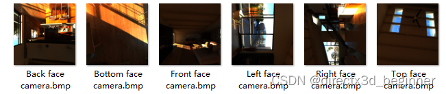
越来越接近真相了。我们很自然地想到，如果把漫游器放在中心打印，是不是就可以打印整个等距柱状投影图了呢？是的，但是，只是要注意的是，立方体贴图的内部和外部尽管一样，但是还是稍微有点模糊，也可以在外部设置漫游器位置六次，打印六次，就像上节那样。但是，这里不考虑这些细节。
也就是把漫游器位置设置为
osg::Vec3d newEye(0, 0, 0);

运行结果不出所料。
在这里插入图片描述

当然，也可以把osg::Image和osg::TextureCubeMap关联起来。使用osg::TextureCubeMap打印。即

int textureWidth = 512;
int textureHeight = 512;

osg::ref_ptr<osg::TextureCubeMap> texture = new osg::TextureCubeMap;

texture->setTextureSize(textureWidth, textureHeight);
texture->setInternalFormat(GL_RGB);
texture->setFilter(osg::Texture::MIN_FILTER, osg::Texture::LINEAR);
texture->setFilter(osg::Texture::MAG_FILTER, osg::Texture::LINEAR);
texture->setWrap(osg::Texture::WRAP_S, osg::Texture::CLAMP_TO_EDGE);
texture->setWrap(osg::Texture::WRAP_T, osg::Texture::CLAMP_TO_EDGE);
texture->setWrap(osg::Texture::WRAP_R, osg::Texture::CLAMP_TO_EDGE);

各个面关联，比如
camera->attach(osg::Camera::COLOR_BUFFER, texture, 0, osg::TextureCubeMap::POSITIVE_Y);

	osg::ref_ptr<osg::Image> printImage = new osg::Image;
	printImage->setFileName(camera->getName());
	printImage->allocateImage(textureWidth, textureHeight, 1, GL_RGBA, GL_UNSIGNED_BYTE);
	texture->setImage(0, printImage);
	camera->attach(osg::Camera::COLOR_BUFFER, printImage);

打印时

		int imageNumber = textureCubeMap->getNumImages(); 
		for (int i = 0; i < imageNumber; i++)
		{

			osg::ref_ptr<osg::Image> theImage = textureCubeMap->getImage(i); 
			std::string strPrintName = "e:/" + theImage->getFileName() + ".bmp";
			osgDB::writeImageFile(* theImage, strPrintName);
		}

完整代码如下：
#include <osg/TextureCubeMap>
#include <osg/TexGen>
#include <osg/TexEnvCombine>
#include <osgUtil/ReflectionMapGenerator>
#include <osgDB/ReadFile>
#include <osgViewer/Viewer>
#include <osg/NodeVisitor>
#include <osg/ShapeDrawable>
#include <osg/Texture2D>
#include <osgGA/TrackballManipulator>
#include <osgDB/WriteFile>
static const char * vertexShader =
{
“in vec3 aPos;\n”
“varying vec3 outPos;”
“void main(void)\n”
“{\n”
“outPos = aPos;\n”
" gl_Position = ftransform();\n"
“}\n”
};

static const char *psShader =
{
“varying vec3 outPos;”
“uniform sampler2D tex0;”
"const vec2 invAtan = vec2(0.1591, 0.3183); "
"vec2 SampleSphericalMap(vec3 v) "
"{ "
" vec2 uv = vec2(atan(v.z, v.x), asin(v.y)); "
" uv *= invAtan; "
" uv += 0.5;

最低0.47元/天解锁文章