


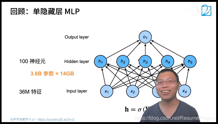

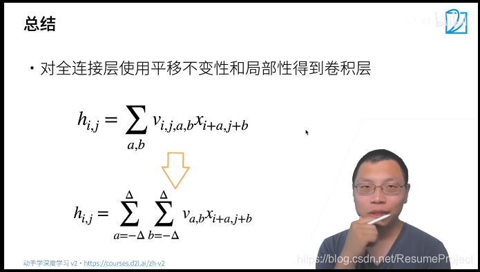
其 实 卷 积 就 是 一 种 特 殊 的 全 连 接 层 下 面 将 从 全 连 接 层 触 发 利 用 这 两 个 原 则 得 到 卷 积 其实卷积就是一种特殊的全连接层\\下面将从全连接层触发利用这两个原则得到卷积 其实卷积就是一种特殊的全连接层下面将从全连接层触发利用这两个原则得到卷积
原
来
是
一
个
二
位
的
矩
阵
乘
以
输
入
的
一
维
向
量
,
现
在
同
理
,
i
,
j
算
是
对
应
轴
的
”
分
裂
“
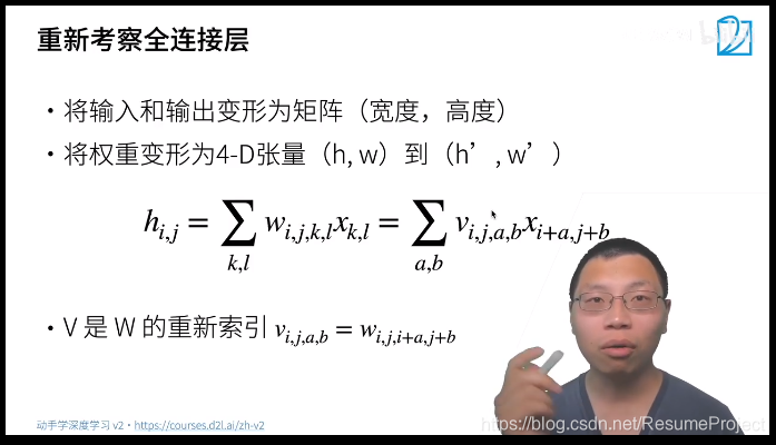
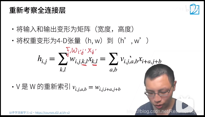
原来是一个二位的矩阵乘以输入的一维向量,现在同理,i,j算是对应轴的”分裂“
原来是一个二位的矩阵乘以输入的一维向量,现在同理,i,j算是对应轴的”分裂“
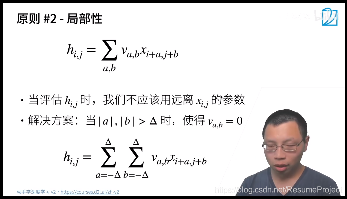
解
决
方
法
:
直
接
抹
掉
前
两
个
维
度
解决方法:直接抹掉前两个维度
解决方法:直接抹掉前两个维度
我
们
称
其
为
2
维
卷
积
,
其
实
是
一
个
误
会
啊
,
在
数
学
上
称
为
2
维
交
叉
相
关
(
其
实
是
在
做
内
积
)
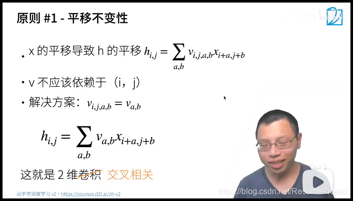
\textcolor{red} {我们称其为2维卷积,其实是一个误会啊,在数学上称为2维交叉相关(其实是在做内积)}
我们称其为2维卷积,其实是一个误会啊,在数学上称为2维交叉相关(其实是在做内积)
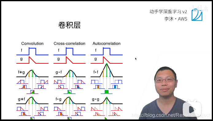
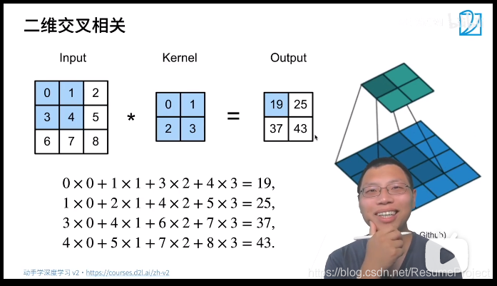
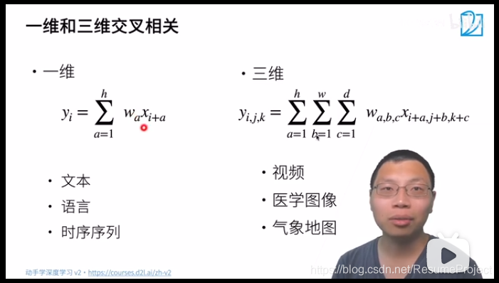
因 为 参 数 W 是 通 过 学 习 产 生 的 , 二 维 交 叉 与 二 维 卷 积 学 出 来 的 W 是 对 称 的 , 但 在 实 际 使 用 中 就 没 有 区 别 了 因为参数W是通过学习产生的,\\二维交叉与二维卷积学出来的W是对称的,但在实际使用中就没有区别了 因为参数W是通过学习产生的,二维交叉与二维卷积学出来的W是对称的,但在实际使用中就没有区别了

卷积层的两个控制大小的超参数:填充&步幅
输入输出计算公式
W o u t = W i n − K e r n a l + 2 P a d d i n g S t e p + 1 W_{out}=\frac{W_{in}-Kernal+2Padding}{Step}+1 Wout=StepWin−Kernal+2Padding+1
输入/输出通道
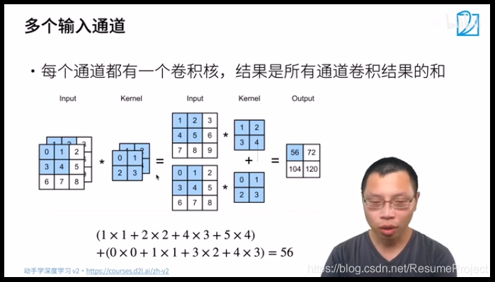
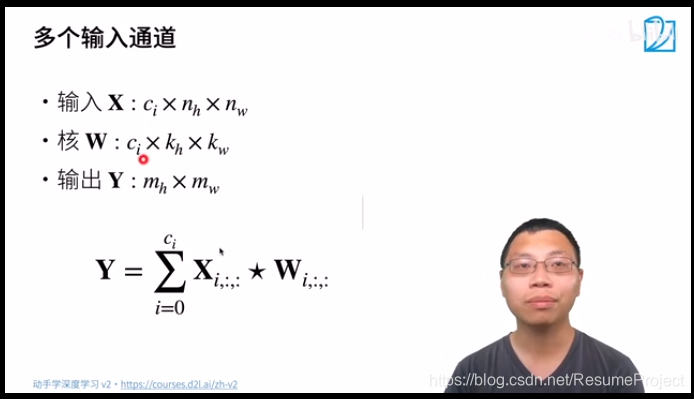
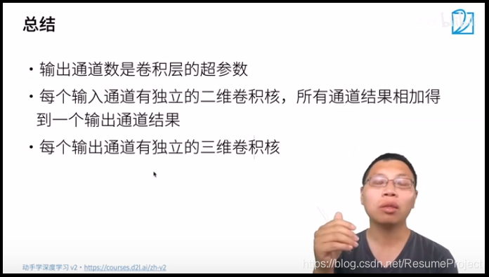
另一个非常常用的超参数:通道数

c
i
维
通
道
数
c_i维通道数
ci维通道数
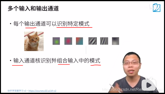
如果多个输出通道呢?
对 于 每 个 输 入 通 道 , 对 应 着 一 个 c o 维 卷 积 核 , 通 过 三 维 卷 积 输 出 , 如 下 , 卷 积 核 多 了 一 个 c o 对于每个输入通道,对应着一个c_o维卷积核,通过三维卷积输出,\\如下,卷积核多了一个c_o 对于每个输入通道,对应着一个co维卷积核,通过三维卷积输出,如下,卷积核多了一个co

[
3
,
8
,
8
]
[
4
,
3
,
3
,
3
]
→
[
4
,
6
,
6
]
[3,8,8] \ \ \ \overrightarrow{\tiny [4,3,3,3]} \ \ \ [4,6,6]
[3,8,8] [4,3,3,3] [4,6,6]
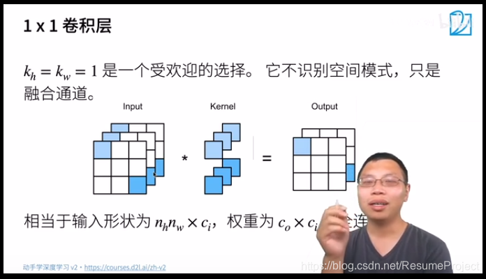
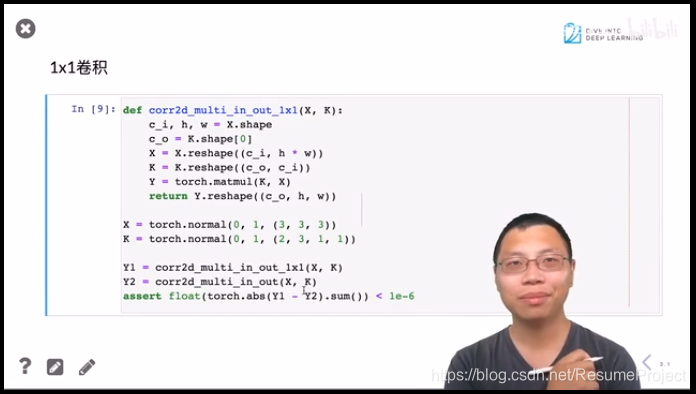
验 证 一 下 1 乘 以 1 的 卷 积 等 价 于 全 联 通 验证一下1乘以1的卷积等价于全联通 验证一下1乘以1的卷积等价于全联通
分组卷积/群卷积(Group Convolution)
以上为普通卷积,以下为分组卷积:群卷积神经网络
Depthwise卷积与Pointwise卷积
nn.MaxPool2d(3, stride=2)
池化层
可分离卷积
https://wjrsbu.smartapps.cn/zhihu/answer?id=615115629&isShared=1&_swebfr=1
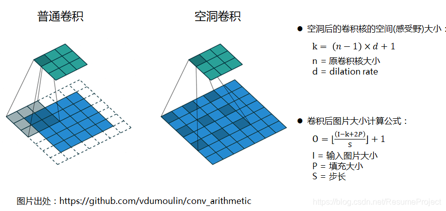
、增大感受野
所谓感受野,即一个像素对应回原图的区域大小,假如没有pooling,一个33,步长为1的卷积,那么输出的一个像素的感受野就是33的区域,再加一个stride=1的33卷积,则感受野为55。
假如我们在每一个卷积中间加上3*3的pooling呢?很明显感受野迅速增大,这就是pooling的一大用处。感受野的增加对于模型的能力的提升是必要的,正所谓“一叶障目则不见泰山也”。
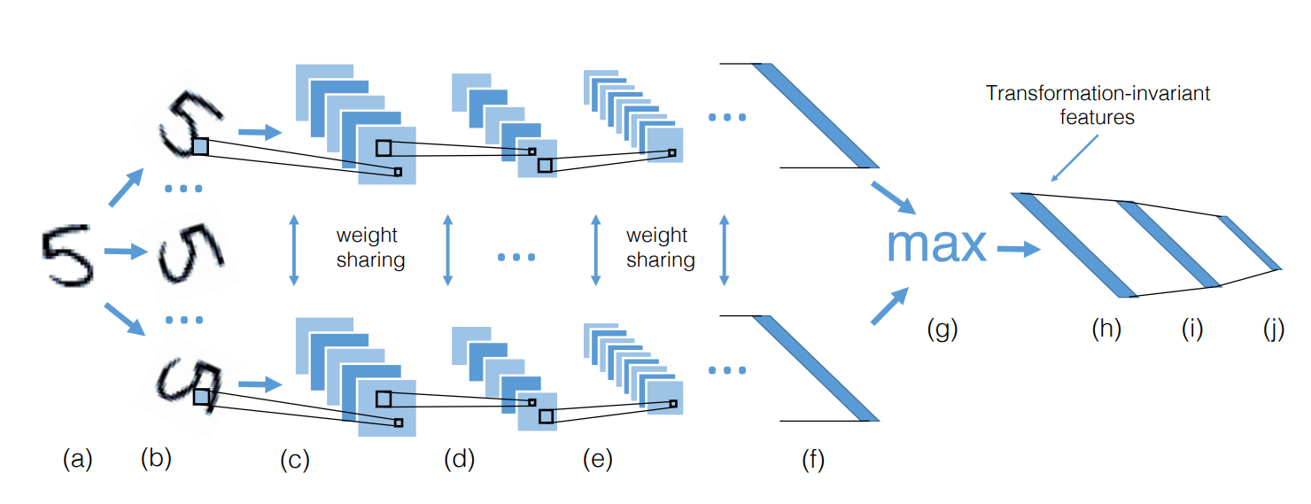
2、平移不变性
我们希望目标的些许位置的移动,能得到相同的结果。因为pooling不断地抽象了区域的特征而不关心位置,所以pooling一定程度上增加了平移不变性。
3、降低优化难度和参数
我们可以用步长大于1的卷积来替代池化,但是池化每个特征通道单独做降采样,与基于卷积的降采样相比,不需要参数,更容易优化。全局池化更是可以大大降低模型的参数量和优化工作量。
stochastic pooling对feature map中的元素按照其概率值大小随机选择,元素被选中的概率与其数值大小正相关,这就是一种正则化的操作了。mixed pooling就是在max/average pooling中进行随机选择。
上面的这些方法都是手动设计,而现在深度学习各个领域其实都是往自动化的方向发展。
我们前面也说过,从激活函数到归一化都开始研究数据驱动的方案,池化也是如此,每一张图片都可以学习到最适合自己的池化方式。
此外还有一些变种如weighted max pooling,Lp pooling,generalization max pooling就不再提了,还有global pooling。
完整解读可移步:龙鹏:【AI初识境】被Hinton,DeepMind和斯坦福嫌弃的池化(pooling),到底是什么?
https://www.cnblogs.com/xxmrecord/p/15170493.html
-条形卷积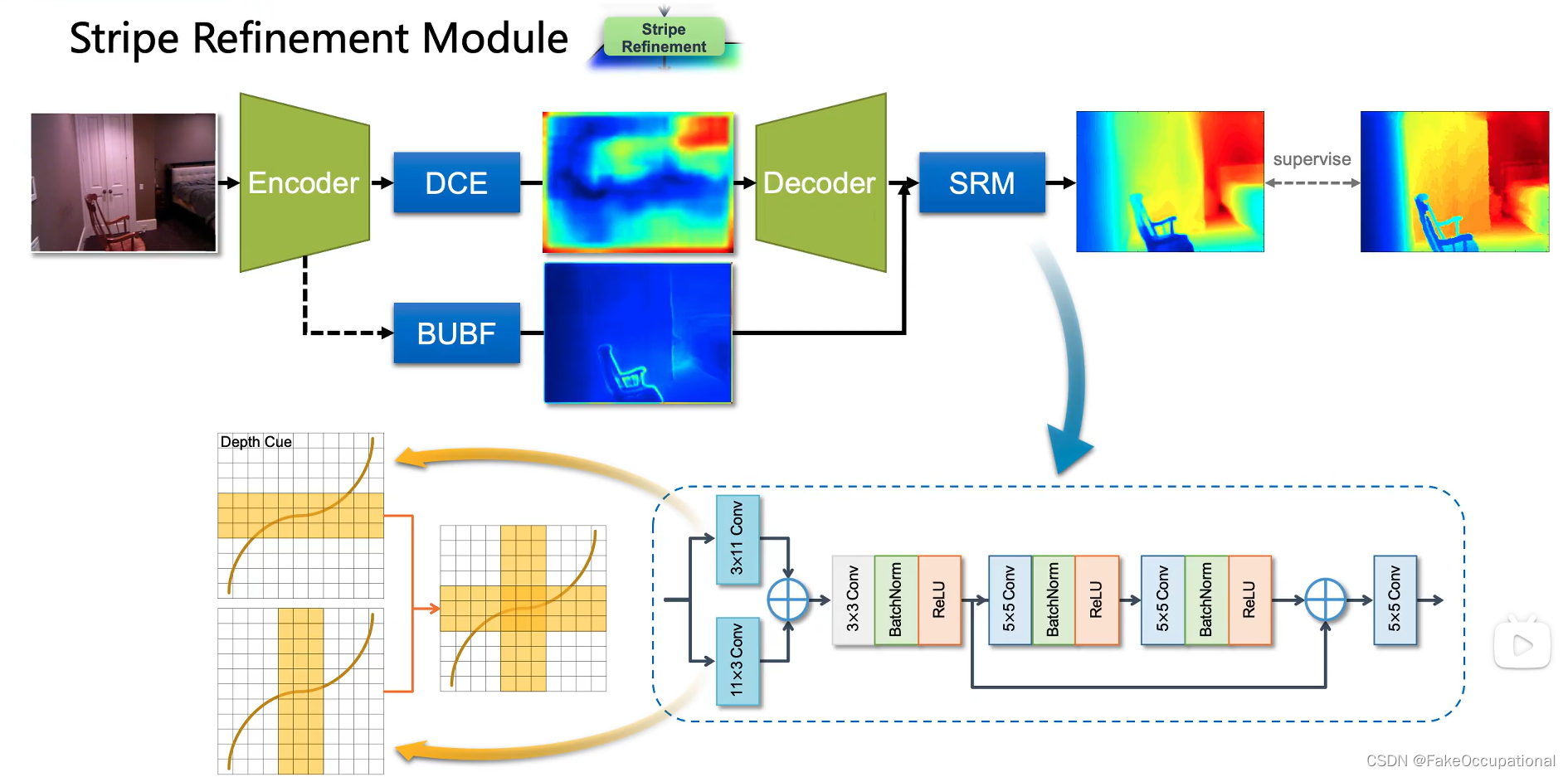
CNN代码(下载数据可能要关闭vpn)
# import some dependencies  https://boscoj2008.github.io/customCNN/
import torchvision
import torch
import torchvision.transforms as transforms
import numpy as np
import matplotlib.pyplot as plt

import torch.optim as optim
import time
import torch.nn as nn
import torch.nn.functional as F
torch.set_printoptions(linewidth=120)


# import data
train_set = torchvision.datasets.FashionMNIST(root="./", download=True,
                                              train=True,
                                              transform=transforms.Compose([transforms.ToTensor()]))

test_set = torchvision.datasets.FashionMNIST(root="./", download=True,
                                              train=False,
                                              transform=transforms.Compose([transforms.ToTensor()]))

data_loader = torch.utils.data.DataLoader(train_set, batch_size=10, shuffle=True,num_workers=0)
sample = next(iter(data_loader))

imgs, lbls = sample


# define some helper functions
def get_item(preds, labels):
    """function that returns the accuracy of our architecture"""
    return preds.argmax(dim=1).eq(labels).sum().item()


@torch.no_grad()  # turn off gradients during inference for memory effieciency
def get_all_preds(network, dataloader):
    """function to return the number of correct predictions across data set"""
    all_preds = torch.tensor([])
    model = network
    for batch in dataloader:
        images, labels = batch
        preds = model(images)  # get preds
        all_preds = torch.cat((all_preds, preds), dim=0)  # join along existing axis

    return all_preds

def plot_confusion_matrix(cm,
                          target_names,
                          title='Confusion matrix',
                          cmap=None,
                          normalize=True):
    """
    given a sklearn confusion matrix (cm), make a nice plot

    Arguments
    ---------
    cm:           confusion matrix from sklearn.metrics.confusion_matrix

    target_names: given classification classes such as [0, 1, 2]
                  the class names, for example: ['high', 'medium', 'low']

    title:        the text to display at the top of the matrix

    cmap:         the gradient of the values displayed from matplotlib.pyplot.cm
                  see http://matplotlib.org/examples/color/colormaps_reference.html
                  plt.get_cmap('jet') or plt.cm.Blues

    normalize:    If False, plot the raw numbers
                  If True, plot the proportions

    Usage
    -----
    plot_confusion_matrix(cm           = cm,                  # confusion matrix created by
                                                              # sklearn.metrics.confusion_matrix
                          normalize    = True,                # show proportions
                          target_names = y_labels_vals,       # list of names of the classes
                          title        = best_estimator_name) # title of graph

    Citiation
    ---------
    http://scikit-learn.org/stable/auto_examples/model_selection/plot_confusion_matrix.html

    """
    import matplotlib.pyplot as plt
    import numpy as np
    import itertools

    accuracy = np.trace(cm) / np.sum(cm).astype('float')
    misclass = 1 - accuracy

    if cmap is None:
        cmap = plt.get_cmap('Blues')

    plt.figure(figsize=(15, 10))
    plt.imshow(cm, interpolation='nearest', cmap=cmap)
    plt.title(title)
    plt.colorbar()

    if target_names is not None:
        tick_marks = np.arange(len(target_names))
        plt.xticks(tick_marks, target_names, rotation=45)
        plt.yticks(tick_marks, target_names)

    if normalize:
        cm = cm.astype('float') / cm.sum(axis=1)[:, np.newaxis]


    thresh = cm.max() / 1.5 if normalize else cm.max() / 2
    for i, j in itertools.product(range(cm.shape[0]), range(cm.shape[1])):
        if normalize:
            plt.text(j, i, "{:0.4f}".format(cm[i, j]),
                     horizontalalignment="center",
                     color="white" if cm[i, j] > thresh else "black")
        else:
            plt.text(j, i, "{:,}".format(cm[i, j]),
                     horizontalalignment="center",
                     color="white" if cm[i, j] > thresh else "black")


    plt.tight_layout()
    plt.ylabel('True label')
    plt.xlabel('Predicted label\naccuracy={:0.4f}; misclass={:0.4f}'.format(accuracy, misclass))
    plt.show()


# define network

class Network(nn.Module):  # extend nn.Module class of nn
    def __init__(self):
        super().__init__()  # super class constructor
        self.conv1 = nn.Conv2d(in_channels=1, out_channels=6, kernel_size=(5, 5))
        self.batchN1 = nn.BatchNorm2d(num_features=6)
        self.conv2 = nn.Conv2d(in_channels=6, out_channels=12, kernel_size=(5, 5))
        self.fc1 = nn.Linear(in_features=12 * 4 * 4, out_features=120)
        self.batchN2 = nn.BatchNorm1d(num_features=120)
        self.fc2 = nn.Linear(in_features=120, out_features=60)
        self.out = nn.Linear(in_features=60, out_features=10)

    def forward(self, t):  # implements the forward method (flow of tensors)

        # hidden conv layer
        t = self.conv1(t)
        t = F.max_pool2d(input=t, kernel_size=2, stride=2)
        t = F.relu(t)
        t = self.batchN1(t)

        # hidden conv layer
        t = self.conv2(t)
        t = F.max_pool2d(input=t, kernel_size=2, stride=2)
        t = F.relu(t)

        # flatten
        t = t.reshape(-1, 12 * 4 * 4)
        t = self.fc1(t)
        t = F.relu(t)
        t = self.batchN2(t)
        t = self.fc2(t)
        t = F.relu(t)

        # output
        t = self.out(t)

        return t
cnn_model = Network() # init model
print(cnn_model) # print model structure

# let's also normalize the data for faster convergence

# import data
mean = 0.2859;  std = 0.3530 # calculated using standization from the MNIST itself which we skip in this blog
# train_set = torchvision.datasets.FashionMNIST(root="./", download=True,
#                                               transform=transforms.Compose([transforms.ToTensor(),
#                                                                             transforms.Normalize(mean, std)
#                                                                            ]))
# data_loader = torch.utils.data.DataLoader(train_set, batch_size=100, shuffle=True, num_workers=1)

optimizer = optim.Adam(lr=0.01, params=cnn_model.parameters())
# def train loop

for epoch in range(5):
    start_time = time.time()
    total_correct = 0
    total_loss = 0
    for batch in data_loader:
        imgs, lbls = batch
        preds = cnn_model(imgs)  # get preds
        loss = F.cross_entropy(preds, lbls)  # compute loss
        optimizer.zero_grad()  # zero grads
        loss.backward()  # calculates gradients
        optimizer.step()  # update the weights

        total_loss += loss.item()
        total_correct += get_item(preds, lbls)
        accuracy = total_correct / len(train_set)
    end_time = time.time() - start_time
    print("Epoch no.", epoch + 1, "|accuracy: ", round(accuracy, 3), "%", "|total_loss: ", total_loss,
          "| epoch_duration: ", round(end_time, 2), "sec")


 1606
1606

 被折叠的 条评论
为什么被折叠?
被折叠的 条评论
为什么被折叠?
 到【灌水乐园】发言


