利用Matlab进行仿真实验，运用卡尔曼滤波实现5G+GNSS松组合

最新推荐文章于 2025-08-04 10:07:39 发布

卫星导航学习者

最新推荐文章于 2025-08-04 10:07:39 发布

阅读量881

点赞数 25

CC 4.0 BY-SA版权

文章标签： matlab 5G gnss 卡尔曼滤波仿真

本文链接：https://blog.youkuaiyun.com/weixin_61546541/article/details/147987392

前言

最近在研究卡尔曼滤波，发现网上关于利用卡尔曼滤波做5G和GNSS融合的帖子较少，因此手搓了一个简易的仿真代码，主要用于学习卡尔曼滤波并进行简单的5G+GNSS融合处理，其中仿真设置较为理想化，有错漏之处还请多多包含。

卡尔曼滤波

作为非常经典和常用的方法，具体原理网上教程也很多，就不赘述了，下面将几个主要公式和含义进行介绍，以方便对代码进行对应。

状态方程：

其中，x为状态变量，x=[ x y z Vx Vy Vz]T，其中x y z为三维坐标，Vx Vy Vz为三维速度。xk是目标在时间k的状态向量，Fk是状态转移矩阵，Gk是控制输入矩阵，uk是控制输入向量，wk是过程噪声。

观测方程可以表示为：

其中，zk是观测向量（GNSS和5G的定位数据，包含位置信息）；Hk是观测矩阵，将状态向量映射到观测空间，vk是观测噪声。

卡尔曼滤波的迭代过程包括预测和更新两个步骤，其中预测步骤是通过状态方程预测下一个时间点的状态：

计算预测误差协方差：

更新步骤是通过预测数据更新状态估计：

更新状态估计：

其中，Qk是过程噪声协方差矩阵，Rk是观测噪声协方差矩阵，Kk是卡尔曼增益。

先给出总的参数设置，后面也会讲到，设置uk=0，P0 =100I6，Qk=0.01I6，Rk=29I3，Hk= [I3 03]，Fk=[I3,I3;03,I3]。

仿真设置

轨迹生成

clc;
clear;
close all;

%% 模拟参数
num_steps = 100;       % 仿真步数
dt = 1;                % 时间间隔（秒）

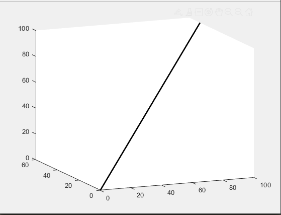
true_pos = [linspace(0, 100, num_steps);  % X坐标从0到100米
            linspace(0, 50, num_steps);   % Y坐标从0到50米
            linspace(0, 100, num_steps)]; % Z坐标从0到100米

这里给出了真实轨迹的生成方式，主要采取了线性化取点的方式，轨迹设置比较简单，有其他需要的可以采用更为复杂的取点方式，轨迹生成图如下：

5G基站位置和GNSS卫星设置

%% 传感器位置（GNSS和5G均为8个点）
% GNSS卫星位置
gnss_pos = [0, 100, 50, 80, 120, 60, 30, 90;
           100, 0, 0, 80, 20, 40, 60, 30;
            30, 30, 60, 10, 50, 70, 40, 20];

% 5G基站位置
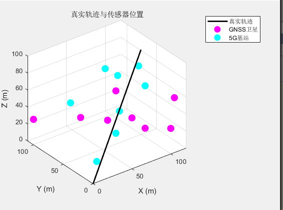
bs_pos = [20, 60, 80, 40, 100, 120, 90, 70;
          20, 40, 60, 90, 110, 80, 30, 50;
          10, 20, 30, 40, 50, 60, 70, 80];

经过挑选，设置了8组卫星和5G基站位置，列为一组数据的X,Y,Z三轴坐标点，其分布如下：

GDOP（Geometric Dilution of Precision，几何精度因子）是衡量卫星导航系统（如 GPS、北斗）中卫星几何分布对定位精度影响的关键指标。其核心原理是：卫星在空间中的几何分布越分散，定位精度越高；分布越集中（如共线或共面），定位误差越大。GDOP的数值越低，代表此时卫星等的空间构型更好，对于定位精度帮助越高。

计算原理如下所示：

%% GDOP计算函数
function gdop = calculate_gdop(anchor_pos, user_pos)
    num_anchors = size(anchor_pos, 2);
    G = zeros(num_anchors, 4);  % 几何矩阵
    
    for i = 1:num_anchors
        dx = anchor_pos(1,i) - user_pos(1);
        dy = anchor_pos(2,i) - user_pos(2);
        dz = anchor_pos(3,i) - user_pos(3);
        dist = norm([dx; dy; dz]);
        
        % 填充几何矩阵
        G(i,1) = dx / dist;
        G(i,2) = dy / dist;
        G(i,3) = dz / dist;
        G(i,4) = 1;  % 钟差项
    end
    
    % 计算位置精度因子
    Q = inv(G' * G);  % 精度矩阵
    gdop = sqrt(trace(Q));  % GDOP = √(tr(Q))
end

GDOP计算结果如下图：

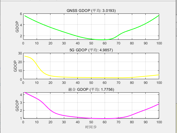
由平均值确定5G基站和GNSS位置选择没有问题，可以满足较好的定位效果。

生成伪距测量（带噪声）

%% 噪声参数
gnss_noise_std = 5;  % GNSS测量噪声标准差
bs_noise_std = 2;    % 5G测量噪声标准差

%% 生成伪距测量（带噪声）
gnss_meas = zeros(size(gnss_pos, 2), num_steps);  % 8行×num_steps列
bs_meas = zeros(size(bs_pos, 2), num_steps);      % 8行×num_steps列
gnss_gdop = zeros(1, num_steps);
bs_gdop = zeros(1, num_steps);
fusion_gdop = zeros(1, num_steps);

for t = 1:num_steps
    for i = 1:size(gnss_pos, 2)
        gnss_meas(i, t) = norm(true_pos(:, t) - gnss_pos(:, i)) + gnss_noise_std*randn;
    end
    for i = 1:size(bs_pos, 2)
        bs_meas(i, t) = norm(true_pos(:, t) - bs_pos(:, i)) + bs_noise_std*randn;
    end

通过设置噪声参数，对于每时每刻的载体运动，因为已知5G基站或者GNSS卫星位置，也知道载体位置，而卫星定位本质也是伪距的确认，同时5G定位也有位置测量的方法（TOA），所以可以通过设置测量噪声进行简单模拟，得到带有噪声的位置测量量。

最小二乘法定位函数

位置的确定采用最小二乘法，利用第一个坐标点为锚点，非线性方程转变为AX=B，线性方程进行求解，具体实现如下：

function pos = ls_positioning_3d(anchor_pos, distances)
    num_anchors = size(anchor_pos, 2);
    if num_anchors < 4    % 三维定位至少需要4个锚点
        error('至少需要4个锚点进行三维定位');
    end
    
    A = zeros(num_anchors-1, 3);
    b = zeros(num_anchors-1, 1);
    
    for i = 2:num_anchors
        A(i-1,:) = 2*(anchor_pos(:,i)' - anchor_pos(:,1)');
        b(i-1) = distances(1)^2 - distances(i)^2 + ...
                 sum(anchor_pos(:,i).^2) - sum(anchor_pos(:,1).^2);
    end
    
    pos = A\b;  % 最小二乘解
end

卡尔曼滤波设置

% 状态向量 [x; y; z; vx; vy; vz]
x_lc = [0; 0; 0; 1; 1; 1];
P_lc = eye(6)*100;  % 初始状态协方差矩阵

% 状态转移矩阵（匀速模型）
F = [eye(3), eye(3)*dt;
     zeros(3), eye(3)];

% 过程噪声协方差矩阵
Q = eye(6) * 0.01;  

% 观测矩阵（直接观测位置）
H = [eye(3), zeros(3)];

% 观测噪声协方差矩阵
R_gnss = eye(3) * gnss_noise_std^2;
R_bs = eye(3) * bs_noise_std^2;

% 初始化结果存储
est_lc = zeros(6, num_steps);        % 松耦合估计结果
gnss_only_est = zeros(3, num_steps); % GNSS单独定位结果
bs_only_est = zeros(3, num_steps);   % 5G单独定位结果
gnss_weight = zeros(1, num_steps);   % GNSS权重
bs_weight = zeros(1, num_steps);     % 5G权重、

卡尔曼滤波主循环

for t = 1:num_steps
    % 基于最小二乘法的位置估计
    gnss_est = ls_positioning_3d(gnss_pos, gnss_meas(:, t));
    bs_est = ls_positioning_3d(bs_pos, bs_meas(:, t));
    
    % 保存单独的估计结果
    gnss_only_est(:, t) = gnss_est;
    bs_only_est(:, t) = bs_est;
    
    % 基于噪声水平的自适应权重计算
    total_uncertainty = gnss_noise_std^2 + bs_noise_std^2;
    gnss_weight(t) = bs_noise_std^2 / total_uncertainty;  % GNSS权重
    bs_weight(t) = gnss_noise_std^2 / total_uncertainty;  % 5G权重
    
    % 加权融合观测值
    z = gnss_weight(t) * gnss_est + bs_weight(t) * bs_est;
    
    % 卡尔曼滤波预测步骤
    x_lc = F * x_lc;
    P_lc = F * P_lc * F' + Q;

    % 卡尔曼滤波更新步骤
    y = z - H * x_lc;
    R_lc = (gnss_weight(t)^2 * R_gnss + bs_weight(t)^2 * R_bs);
    S = H * P_lc * H' + R_lc;
    K = P_lc * H' / S;
    x_lc = x_lc + K * y;
    P_lc = (eye(6) - K * H) * P_lc;

    % 保存当前时刻的状态估计
    est_lc(:, t) = x_lc;
end

这里采用了加权的卡尔曼滤波，根据噪声量的不同对测量值进行权重分配，以衡量测量值的可信度。

具体输出如下：

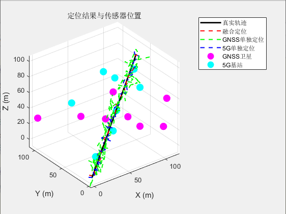
误差分析如下：

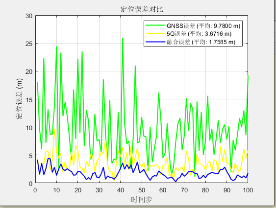
可以看出相较于单独GNSS和5G定位，融合定位误差更低，滤波效果符合预期。

附录（完整代码）

下面是完整代码，想要下载的也可以前往：

【免费】利用卡尔曼滤波进行5G+GNSS松耦合资源-优快云文库

clc;
clear;
close all;

%% 模拟参数
num_steps = 100;       % 仿真步数
dt = 1;                % 时间间隔（秒）

%% 轨迹生成
% 真实轨迹（匀速直线运动 三维）
true_pos = [linspace(0, 100, num_steps);  % X坐标从0到100米
            linspace(0, 50, num_steps);   % Y坐标从0到50米
            linspace(0, 100, num_steps)]; % Z坐标从0到100米

%% 传感器位置（GNSS和5G均为8个点）
% GNSS卫星位置
gnss_pos = [0, 100, 50, 80, 120, 60, 30, 90;
           100, 0, 0, 80, 20, 40, 60, 30;
            30, 30, 60, 10, 50, 70, 40, 20];

% 5G基站位置
bs_pos = [20, 60, 80, 40, 100, 120, 90, 70;
          20, 40, 60, 90, 110, 80, 30, 50;
          10, 20, 30, 40, 50, 60, 70, 80];

%% 噪声参数
gnss_noise_std = 5;  % GNSS测量噪声标准差
bs_noise_std = 2;    % 5G测量噪声标准差

%% 生成伪距测量（带噪声）
gnss_meas = zeros(size(gnss_pos, 2), num_steps);  % 8行×num_steps列
bs_meas = zeros(size(bs_pos, 2), num_steps);      % 8行×num_steps列
gnss_gdop = zeros(1, num_steps);
bs_gdop = zeros(1, num_steps);
fusion_gdop = zeros(1, num_steps);

for t = 1:num_steps
    for i = 1:size(gnss_pos, 2)
        gnss_meas(i, t) = norm(true_pos(:, t) - gnss_pos(:, i)) + gnss_noise_std*randn;
    end
    for i = 1:size(bs_pos, 2)
        bs_meas(i, t) = norm(true_pos(:, t) - bs_pos(:, i)) + bs_noise_std*randn;
    end
    
    % 计算几何精度因子(GDOP)
    gnss_gdop(t) = calculate_gdop(gnss_pos, true_pos(:, t));
    bs_gdop(t) = calculate_gdop(bs_pos, true_pos(:, t));
    fusion_gdop(t) = calculate_gdop([gnss_pos, bs_pos], true_pos(:, t));
end

%% 松耦合卡尔曼滤波器
% 状态向量 [x; y; z; vx; vy; vz]
x_lc = [0; 0; 0; 1; 1; 1];
P_lc = eye(6)*100;  % 初始状态协方差矩阵

% 状态转移矩阵（匀速模型）
F = [eye(3), eye(3)*dt;
     zeros(3), eye(3)];

% 过程噪声协方差矩阵
Q = eye(6) * 0.01;  

% 观测矩阵（直接观测位置）
H = [eye(3), zeros(3)];

% 观测噪声协方差矩阵
R_gnss = eye(3) * gnss_noise_std^2;
R_bs = eye(3) * bs_noise_std^2;

% 初始化结果存储
est_lc = zeros(6, num_steps);        % 松耦合估计结果
gnss_only_est = zeros(3, num_steps); % GNSS单独定位结果
bs_only_est = zeros(3, num_steps);   % 5G单独定位结果
gnss_weight = zeros(1, num_steps);   % GNSS权重
bs_weight = zeros(1, num_steps);     % 5G权重

% 卡尔曼滤波主循环
for t = 1:num_steps
    % 基于最小二乘法的位置估计
    gnss_est = ls_positioning_3d(gnss_pos, gnss_meas(:, t));
    bs_est = ls_positioning_3d(bs_pos, bs_meas(:, t));
    
    % 保存单独的估计结果
    gnss_only_est(:, t) = gnss_est;
    bs_only_est(:, t) = bs_est;
    
    % 基于噪声水平的自适应权重计算
    total_uncertainty = gnss_noise_std^2 + bs_noise_std^2;
    gnss_weight(t) = bs_noise_std^2 / total_uncertainty;  % GNSS权重
    bs_weight(t) = gnss_noise_std^2 / total_uncertainty;  % 5G权重
    
    % 加权融合观测值
    z = gnss_weight(t) * gnss_est + bs_weight(t) * bs_est;
    
    % 卡尔曼滤波预测步骤
    x_lc = F * x_lc;
    P_lc = F * P_lc * F' + Q;

    % 卡尔曼滤波更新步骤
    y = z - H * x_lc;
    R_lc = (gnss_weight(t)^2 * R_gnss + bs_weight(t)^2 * R_bs);
    S = H * P_lc * H' + R_lc;
    K = P_lc * H' / S;
    x_lc = x_lc + K * y;
    P_lc = (eye(6) - K * H) * P_lc;

    % 保存当前时刻的状态估计
    est_lc(:, t) = x_lc;
end

%% 误差计算
time = 1:num_steps;
gnss_error = zeros(1, num_steps);
bs_error = zeros(1, num_steps);
lc_error = zeros(1, num_steps);

for t = 1:num_steps
    gnss_error(t) = norm(gnss_only_est(:, t) - true_pos(:, t));
    bs_error(t) = norm(bs_only_est(:, t) - true_pos(:, t));
    lc_error(t) = norm(est_lc(1:3, t) - true_pos(:, t));
end

% 计算统计量
avg_gnss_error = mean(gnss_error);
avg_bs_error = mean(bs_error);
avg_lc_error = mean(lc_error);
avg_gnss_gdop = mean(gnss_gdop);
avg_bs_gdop = mean(bs_gdop);
avg_fusion_gdop = mean(fusion_gdop);

%% 结果可视化
% 图1：融合定位结果与传感器位置
figure(1);
plot3(true_pos(1,:), true_pos(2,:), true_pos(3,:), 'k-', 'LineWidth', 2); hold on;
plot3(est_lc(1,:), est_lc(2,:), est_lc(3,:), 'r--', 'LineWidth', 1.5);
plot3(gnss_only_est(1,:), gnss_only_est(2,:), gnss_only_est(3,:), 'g--', 'LineWidth', 1.5);
plot3(bs_only_est(1,:), bs_only_est(2,:), bs_only_est(3,:), 'b--', 'LineWidth', 1.5);
plot3(gnss_pos(1,:), gnss_pos(2,:), gnss_pos(3,:), 'mo', 'MarkerSize', 10, 'MarkerFaceColor', 'm');
plot3(bs_pos(1,:), bs_pos(2,:), bs_pos(3,:), 'co', 'MarkerSize', 10, 'MarkerFaceColor', 'c');
legend('真实轨迹', '融合定位',  'GNSS单独定位','5G单独定位','GNSS卫星', '5G基站');
xlabel('X (m)'); ylabel('Y (m)'); zlabel('Z (m)');
title('定位结果与传感器位置');
grid on; axis equal;

% 图2：GNSS单独定位结果
figure(2);
plot3(true_pos(1,:), true_pos(2,:), true_pos(3,:), 'k-', 'LineWidth', 2); hold on;
plot3(gnss_only_est(1,:), gnss_only_est(2,:), gnss_only_est(3,:), 'g--', 'LineWidth', 1.5);
plot3(gnss_pos(1,:), gnss_pos(2,:), gnss_pos(3,:), 'mo', 'MarkerSize', 10, 'MarkerFaceColor', 'm');
legend('真实轨迹', 'GNSS定位', 'GNSS卫星');
xlabel('X (m)'); ylabel('Y (m)'); zlabel('Z (m)');
title('GNSS单独定位结果');
grid on; axis equal;

% 图3：5G单独定位结果
figure(3);
plot3(true_pos(1,:), true_pos(2,:), true_pos(3,:), 'k-', 'LineWidth', 2); hold on;
plot3(bs_only_est(1,:), bs_only_est(2,:), bs_only_est(3,:), 'y--', 'LineWidth', 1.5);
plot3(bs_pos(1,:), bs_pos(2,:), bs_pos(3,:), 'co', 'MarkerSize', 10, 'MarkerFaceColor', 'c');
legend('真实轨迹', '5G定位', '5G基站');
xlabel('X (m)'); ylabel('Y (m)'); zlabel('Z (m)');
title('5G单独定位结果');
grid on; axis equal;

% 图4：定位误差对比
figure(4);
plot(time, gnss_error, 'g-', 'LineWidth', 1.5); hold on;
plot(time, bs_error, 'y-', 'LineWidth', 1.5);
plot(time, lc_error, 'b-', 'LineWidth', 1.5);
legend(['GNSS误差 (平均: ' num2str(avg_gnss_error, '%.4f') ' m)'], ...
       ['5G误差 (平均: ' num2str(avg_bs_error, '%.4f') ' m)'], ...
       ['融合误差 (平均: ' num2str(avg_lc_error, '%.4f') ' m)']);
xlabel('时间步'); ylabel('定位误差 (m)');
title('定位误差对比');
grid on;

% 图5：自适应权重变化
figure(5);
plot(time, gnss_weight, 'g-', 'LineWidth', 1.5); hold on;
plot(time, bs_weight, 'c-', 'LineWidth', 1.5);
legend('GNSS权重', '5G权重');
xlabel('时间步'); ylabel('权重');
title('自适应权重变化');
grid on;

% 图6：几何精度因子对比
figure(6);
plot(time, gnss_gdop, 'g-', 'LineWidth', 1.5); hold on;
plot(time, bs_gdop, 'y-', 'LineWidth', 1.5);
plot(time, fusion_gdop, 'm-', 'LineWidth', 1.5);
legend(['GNSS GDOP (平均: ' num2str(avg_gnss_gdop, '%.4f') ')'], ...
       ['5G GDOP (平均: ' num2str(avg_bs_gdop, '%.4f') ')'], ...
       ['融合 GDOP (平均: ' num2str(avg_fusion_gdop, '%.4f') ')']);
xlabel('时间步'); ylabel('GDOP');
title('几何精度因子变化');
grid on;

% 图7：GDOP分离子图
figure(7);
subplot(3,1,1);
plot(time, gnss_gdop, 'g-', 'LineWidth', 1.5);
title(['GNSS GDOP (平均: ' num2str(avg_gnss_gdop, '%.4f') ')']);
ylabel('GDOP');
grid on;

subplot(3,1,2);
plot(time, bs_gdop, 'y-', 'LineWidth', 1.5);
title(['5G GDOP (平均: ' num2str(avg_bs_gdop, '%.4f') ')']);
ylabel('GDOP');
grid on;

subplot(3,1,3);
plot(time, fusion_gdop, 'm-', 'LineWidth', 1.5);
title(['融合 GDOP (平均: ' num2str(avg_fusion_gdop, '%.4f') ')']);
xlabel('时间步');
ylabel('GDOP');
grid on;

% 图8：真实轨迹与传感器位置
figure(8);
plot3(true_pos(1,:), true_pos(2,:), true_pos(3,:), 'k-', 'LineWidth', 2); hold on;
plot3(gnss_pos(1,:), gnss_pos(2,:), gnss_pos(3,:), 'mo', 'MarkerSize', 10, 'MarkerFaceColor', 'm');
plot3(bs_pos(1,:), bs_pos(2,:), bs_pos(3,:), 'co', 'MarkerSize', 10, 'MarkerFaceColor', 'c');
legend('真实轨迹', 'GNSS卫星', '5G基站');
xlabel('X (m)'); ylabel('Y (m)'); zlabel('Z (m)');
title('真实轨迹与传感器位置');
grid on; axis equal;

%% 最小二乘法定位函数
function pos = ls_positioning_3d(anchor_pos, distances)
    num_anchors = size(anchor_pos, 2);
    if num_anchors < 4    % 三维定位至少需要4个锚点
        error('至少需要4个锚点进行三维定位');
    end
    
    A = zeros(num_anchors-1, 3);
    b = zeros(num_anchors-1, 1);
    
    for i = 2:num_anchors
        A(i-1,:) = 2*(anchor_pos(:,i)' - anchor_pos(:,1)');
        b(i-1) = distances(1)^2 - distances(i)^2 + ...
                 sum(anchor_pos(:,i).^2) - sum(anchor_pos(:,1).^2);
    end
    
    pos = A\b;  % 最小二乘解
end

%% GDOP计算函数
function gdop = calculate_gdop(anchor_pos, user_pos)
    num_anchors = size(anchor_pos, 2);
    G = zeros(num_anchors, 4);  % 几何矩阵
    
    for i = 1:num_anchors
        dx = anchor_pos(1,i) - user_pos(1);
        dy = anchor_pos(2,i) - user_pos(2);
        dz = anchor_pos(3,i) - user_pos(3);
        dist = norm([dx; dy; dz]);
        
        % 填充几何矩阵
        G(i,1) = dx / dist;
        G(i,2) = dy / dist;
        G(i,3) = dz / dist;
        G(i,4) = 1;  % 钟差项
    end
    
    % 计算位置精度因子
    Q = inv(G' * G);  % 精度矩阵
    gdop = sqrt(trace(Q));  % GDOP = √(tr(Q))
end