【opencv450 Image Processing】Histogram Equalization 直方图均衡化

Goal

在本教程中，您将学习：

什么是图像直方图以及它为何有用

使用 OpenCV 函数 cv::equalizeHist 均衡图像的直方图

Theory

什么是图像直方图？Image Histogram

它是图像强度分布的图形表示。

它量化了所考虑的每个强度值的像素数。

• It is a graphical representation of the intensity distribution of an image.
• It quantifies the number of pixels for each intensity value considered.

 

什么是直方图均衡？Histogram Equalization

这是一种提高图像对比度的方法，以扩展强度范围（另请参见相应的 Wikipedia 条目）。

为了更清楚，从上图中，您可以看到像素似乎聚集在可用强度范围的中间。 直方图均衡所做的就是扩大这个范围。 看看下图：绿色圆圈表示 underpopulated人口不足的强度。 应用均衡后，我们得到一个像中间图一样的直方图。 生成的图像如右图所示。

 

How does it work?

它是如何工作的？

均衡意味着将一个分布（给定的直方图）映射到另一个分布（强度值的更广泛和更均匀的分布），因此强度值分布在整个范围内。

为了达到均衡效果，重映射应该是累积分布函数（cdf）（更多细节请参考学习OpenCV）。 对于直方图 H(i)，其累积分布 H′(i) 为：

 

要将其用作重映射函数，我们必须对 H'(i) 进行归一化，使其最大值为 255（或图像强度的最大值）。 从上面的例子中，累积函数是：

 

最后，我们使用一个简单的重映射程序来获得均衡图像的强度值：

 

Code

这个程序有什么作用？

加载图像

将原始图像转换为灰度

使用 OpenCV 函数 cv::equalizeHist 均衡直方图

在窗口中显示源图像和均衡图像。

可下载代码：点击这里opencv/EqualizeHist_Demo.cpp at 4.x · opencv/opencv (github.com)

代码一览：

/**
 * @function EqualizeHist_Demo.cpp
 * @brief 直方图均衡化Demo code for equalizeHist function
 * @author OpenCV team
 */

#include "opencv2/imgcodecs.hpp"
#include "opencv2/highgui.hpp"
#include "opencv2/imgproc.hpp"
#include <iostream>

using namespace cv;
using namespace std;

/**
 * @function main
 */
int main( int argc, char** argv )
{
    //! [加载图像]
    CommandLineParser parser( argc, argv, "{@input | lena.jpg | input image}" );
    Mat src = imread( samples::findFile( parser.get<String>( "@input" ) ), IMREAD_COLOR );
    if( src.empty() )
    {
        cout << "Could not open or find the image!\n" << endl;
        cout << "Usage: " << argv[0] << " <Input image>" << endl;
        return -1;
    }
    //! [Load image]

    //! [转换为灰度图]
    cvtColor( src, src, COLOR_BGR2GRAY );
    //! [Convert to grayscale]

    //! [应用直方图均衡]
    Mat dst;
    equalizeHist( src, dst );
    //! [Apply Histogram Equalization]

    //! [显示结果]
    imshow( "Source image", src );
    imshow( "Equalized Image", dst );
    //! [Display results]

    //! [Wait until user exits the program]
    waitKey();
    //! [Wait until user exits the program]

    return 0;

}

Explanation

加载源图像：

CommandLineParser parser( argc, argv, "{@input | lena.jpg | input image}" );
Mat src = imread( samples::findFile( parser.get<String>( "@input" ) ), IMREAD_COLOR );
if( src.empty() )
{
cout << "Could not open or find the image!\n" << endl;
cout << "Usage: " << argv[0] << " <Input image>" << endl;
return -1;
}

• Convert it to grayscale:

cvtColor( src, src, COLOR_BGR2GRAY );

• Apply histogram equalization with the function cv::equalizeHist :

直方图均衡

Mat dst;
equalizeHist( src, dst );

很容易看出，唯一的参数是原始图像和输出（均衡）图像。

显示两个图像（原始和均衡）：

imshow( "Source image", src );
imshow( "Equalized Image", dst );

等到用户退出程序

waitKey();

Results

1. 为了更好地欣赏均衡的效果，我们引入一张对比度不大的图像，例如：

 

顺便说一下，它有这个直方图：

 

请注意，像素聚集在直方图的中心周围。

1. 在我们的程序应用均衡后，我们得到这个结果：

 

这个图像肯定有更多的对比度。 查看它的新直方图，如下所示：

 

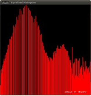
请注意像素数如何在强度范围内分布得更均匀。