


1、主要参考
(1)github地址
ComputerVision/monocularDepth.py at master · niconielsen32/ComputerVision · GitHub
(2)Midas模型的地址
GitHub - isl-org/MiDaS: Code for robust monocular depth estimation described in "Ranftl et. al., Towards Robust Monocular Depth Estimation: Mixing Datasets for Zero-shot Cross-dataset Transfer, TPAMI 2022" (3)Midas pytorch.hub百度下载地址,大佬的blog
机器学习笔记 - 基于Torch Hub的深度估计模型MiDaS_坐望云起的博客-优快云博客_midas 深度估计
(4)重要参考,转onnx
成功将Midas模型转换为ONNX后出现ONNX运行时测试错误 - 问答 - Python中文网
(5)python生成棋盘格
Python图像拼接之自定义生成棋盘格_Thomson617的博客-优快云博客
(6)内参矩阵解析
【OpenCV】OpenCV-Python实现相机标定+利用棋盘格相对位姿估计_Quentin_HIT的博客-优快云博客_opencv python 棋盘格
2、生成棋盘格
(1)直接参考了大佬的代码
Python图像拼接之自定义生成棋盘格_Thomson617的博客-优快云博客
(2)具体代码如下
#代码来源
#https://blog.youkuaiyun.com/Thomson617/article/details/104022558
# -*- coding:utf-8 -*-
import cv2
import numpy as np
def generatePattern(CheckerboardSize, Nx_cor, Ny_cor):
'''
自定义生成棋盘
:param CheckerboardSize: 棋盘格大小,此处100即可
:param Nx_cor: 棋盘格横向内角数
:param Ny_cor: 棋盘格纵向内角数
:return:
'''
black = np.zeros((CheckerboardSize, CheckerboardSize, 3), np.uint8)
white = np.zeros((CheckerboardSize, CheckerboardSize, 3), np.uint8)
black[:] = [0, 0, 0] # 纯黑色
white[:] = [255, 255, 255] # 纯白色
black_white = np.concatenate([black, white], axis=1)
black_white2 = black_white
white_black = np.concatenate([white, black], axis=1)
white_black2 = white_black
# 横向连接
if Nx_cor % 2 == 1:
for i in range(1, (Nx_cor+1) // 2):
black_white2 = np.concatenate([black_white2, black_white], axis=1)
white_black2 = np.concatenate([white_black2, white_black], axis=1)
else:
for i in range(1, Nx_cor // 2):
black_white2 = np.concatenate([black_white2, black_white], axis=1)
white_black2 = np.concatenate([white_black2, white_black], axis=1)
black_white2 = np.concatenate([black_white2, black], axis=1)
white_black2 = np.concatenate([white_black2, white], axis=1)
jj = 0
black_white3 = black_white2
for i in range(0, Ny_cor):
jj += 1
# 纵向连接
if jj % 2 == 1:
black_white3 = np.concatenate((black_white3, white_black2)) # =np.vstack((img1, img2))
else:
black_white3 = np.concatenate((black_white3, black_white2)) # =np.vstack((img1, img2))
cv2.imshow('', black_white3)
cv2.imwrite('pattern.jpg', black_white3)
cv2.waitKey(5000)
cv2.destroyAllWindows()
if __name__ == '__main__':
# generatePattern(100, 9, 6)
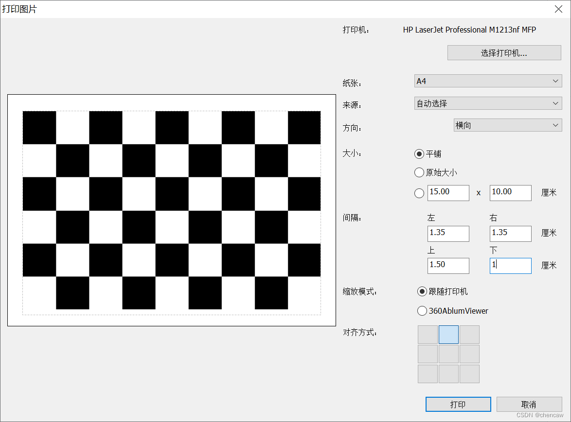
generatePattern(100, 8, 5)(3)用激光打印机打印一下,的3cm*3cm大小的棋盘格
简单的计算一下,打印即可
3、捕获图片
(1)编写简单的代码捕获图片
#加载opencv模块
import cv2 as cv

#获取摄像头
cap = cv.VideoCapture(1)
count = 0
savepath = 'D:/RGBD_CAMERA/python_3d_process/1mono_to_3d/images/'
print("start")
while (cap.isOpened()):
    ret, frame = cap.read() #捕获图片
    if ret == False:
        break
    frame = cv.flip(frame,1)    #镜像操作
    cv.imshow("video", frame)
    key = cv.waitKey(30)
    if key  == ord('q'):  #如果是按键q,则退出
        break
    if key  == ord('r'):  #如果是按键r,则记录
        count = count+1
        cv.imwrite(savepath+str(count)+'.jpg',frame)

cap.release()
cv.destroyAllWindows()
(2)注意:采集图片的数量建议超过12张
4、标定
(1)代码
import cv2
import numpy as np
import glob


savepath = 'D:/RGBD_CAMERA/python_3d_process/1mono_to_3d/images/'
# 找棋盘格角点
# 设置寻找亚像素角点的参数,采用的停止准则是最大循环次数30和最大误差容限0.001
criteria = (cv2.TERM_CRITERIA_EPS + cv2.TERM_CRITERIA_MAX_ITER, 30, 0.001) # 阈值

#棋盘格模板规格
# w = 9   # 10 - 1
# h = 9   # 10  - 1
w = 8   # 9 - 1
h = 5   # 6  - 1

#实际打印方格尺寸
real_size = 30  #mm
# 世界坐标系中的棋盘格点,例如(0,0,0), (1,0,0), (2,0,0) ....,(8,5,0),去掉Z坐标,记为二维矩阵
objp = np.zeros((w*h,3), np.float32)
objp[:,:2] = np.mgrid[0:w,0:h].T.reshape(-1,2)
# objp = objp*18.1  # 18.1 mm
objp = objp*real_size  # 30 mm

# 储存棋盘格角点的世界坐标和图像坐标对
objpoints = [] # 在世界坐标系中的三维点
imgpoints = [] # 在图像平面的二维点
#加载pic文件夹下所有的jpg图像
# images = glob.glob('./*.jpg')  #   拍摄的十几张棋盘图片所在目录
images = glob.glob(savepath+'*.jpg')  #   拍摄的十几张棋盘图片所在目录

i=0
for fname in images:

    img = cv2.imread(fname)
    # 获取画面中心点
    #获取图像的长宽
    h1, w1 = img.shape[0], img.shape[1]
    gray = cv2.cvtColor(img,cv2.COLOR_BGR2GRAY)
    u, v = img.shape[:2]
    # 找到棋盘格角点
    ret, corners = cv2.findChessboardCorners(gray, (w,h),None)
    # 如果找到足够点对,将其存储起来
    if ret == True:
        print("i:", i)
        i = i+1
        # 在原角点的基础上寻找亚像素角点
        cv2.cornerSubPix(gray,corners,(11,11),(-1,-1),criteria)
        #追加进入世界三维点和平面二维点中
        objpoints.append(objp)
        imgpoints.append(corners)
        # 将角点在图像上显示
        cv2.drawChessboardCorners(img, (w,h), corners, ret)
        cv2.namedWindow('findCorners', cv2.WINDOW_NORMAL)
        cv2.resizeWindow('findCorners', 640, 480)
        cv2.imshow('findCorners',img)
        cv2.waitKey(200)
cv2.destroyAllWindows()

## 标定
print('正在计算')
#标定
ret, mtx, dist, rvecs, tvecs = \
    cv2.calibrateCamera(objpoints, imgpoints, gray.shape[::-1], None, None)


print("ret:",ret  )
print("mtx:\n",mtx)      # 内参数矩阵
print("dist畸变值:\n",dist   )   # 畸变系数   distortion cofficients = (k_1,k_2,p_1,p_2,k_3)
print("rvecs旋转(向量)外参:\n",rvecs)   # 旋转向量  # 外参数
print("tvecs平移(向量)外参:\n",tvecs  )  # 平移向量  # 外参数
newcameramtx, roi = cv2.getOptimalNewCameraMatrix(mtx, dist, (u, v), 0, (u, v))
print('newcameramtx外参',newcameramtx)


#打开摄像机
camera=cv2.VideoCapture(1)
# camera=cv2.VideoCapture(0)
while True:
    (grabbed,frame)=camera.read()
    h1, w1 = frame.shape[:2]
    newcameramtx, roi = cv2.getOptimalNewCameraMatrix(mtx, dist, (u, v), 0, (u, v))
    # 纠正畸变
    dst1 = cv2.undistort(frame, mtx, dist, None, newcameramtx)
    #dst2 = cv2.undistort(frame, mtx, dist, None, newcameramtx)
    mapx,mapy=cv2.initUndistortRectifyMap(mtx,dist,None,newcameramtx,(w1,h1),5)
    dst2=cv2.remap(frame,mapx,mapy,cv2.INTER_LINEAR)
    # 裁剪图像,输出纠正畸变以后的图片
    x, y, w1, h1 = roi
    dst1 = dst1[y:y + h1, x:x + w1]

    #cv2.imshow('frame',dst2)
    #cv2.imshow('dst1',dst1)
    cv2.imshow('dst2', dst2)
    if cv2.waitKey(1) & 0xFF == ord('q'):  # 按q保存一张图片
        cv2.imwrite("../u4/frame.jpg", dst1)
        break

camera.release()
cv2.destroyAllWindows()
(2)得到的内参
mtx:
[[801.31799138 0. 319.96097314]
[ 0. 804.76125593 206.79594003]
[ 0. 0. 1. ]]
dist畸变值:
[[-7.21246445e-02 -6.84714453e-01 -1.25501966e-02 5.75752614e-03
9.50679972e+00]]
(3)内参矩阵参数解析
参考了
【OpenCV】OpenCV-Python实现相机标定+利用棋盘格相对位姿估计_Quentin_HIT的博客-优快云博客_opencv python 棋盘格
内参矩阵的具体表达式如下:
其中,和
分别是每个像素在图像平面
和
方向上的物理尺寸,
是图像坐标系原点在像素坐标系中的坐标,
为摄像头的焦距,
,
为焦距
与像素物理尺寸的比值,单位为个(像素数目)。
- 据此可以得到,这台摄像头的fx约为801,fy约为805,说明焦距fx约等于801个像素的物理尺寸,fy约等于804个像素的物理尺寸。
- u0约为320,v0约为207。这台摄像头当前设定的像素为640×480,因此
的理论值应为320,
的理论值应为240。误差主要是因为摄像头的分辨率太低,实际角点在像素坐标系中显示不准;此外,目标坐标系的测量时也会带来误差。
5、单目深度估计方法
5.1 安装依赖
pip install timm5.2手动下载Midas模型
5.2.1下载模型
(1)参考大佬的blog,好人啊,大家给他点赞!
机器学习笔记 - 基于Torch Hub的深度估计模型MiDaS_坐望云起的博客-优快云博客_midas 深度估计
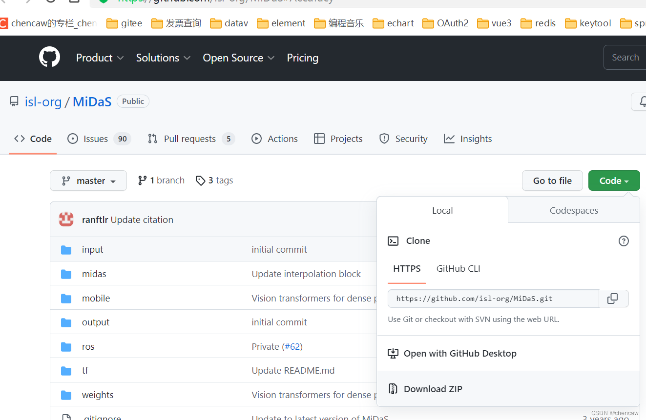
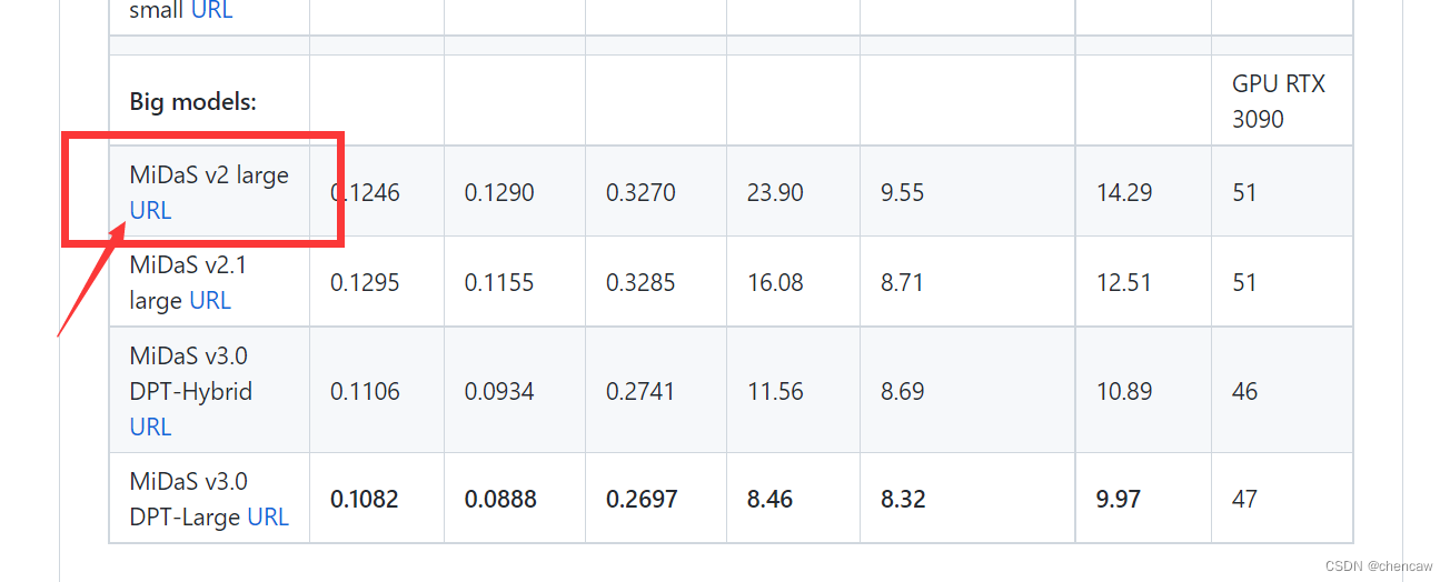
(2)或者直接进github官网地址下载
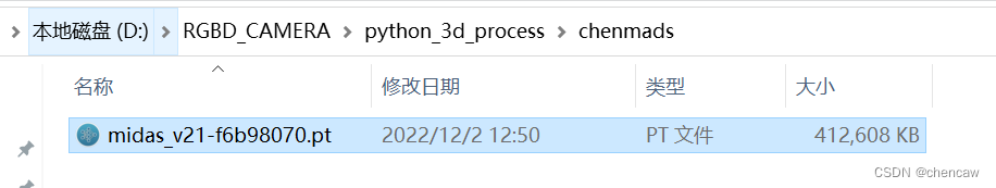
(3)下载的巨大模型
![]()
5.2.2下载代码
(1)进官网下载代码
(2)代码不大,偷懒的话就直接下载zip
(3)解压一下
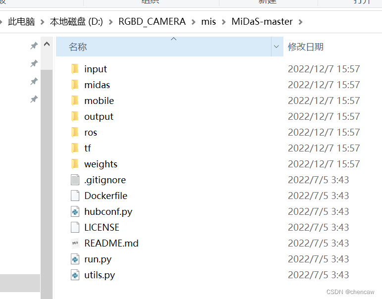
(3)为了本地使用,修改hubconf.py内容
        # state_dict = torch.hub.load_state_dict_from_url(
        #     checkpoint, map_location=torch.device('cpu'), progress=True, check_hash=True
        # )
        state_dict = torch.load('D:/BaiduNetdiskDownload/dpt_large-midas-2f21e586.pt', map_location=torch.device('cpu'))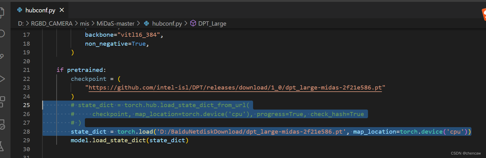
6 单目图像深度估计代码的实现
6.1 细节可以参考pytorch官方的教程(仅供参考)
6.2实际实现
注意:由于torch.hub不好用,所以接着5.2.2的设置测试
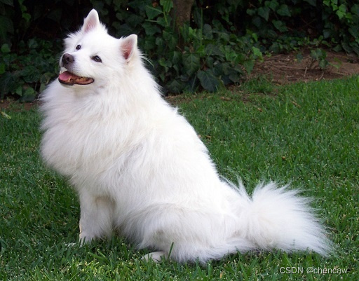
6.3 把测试的dog图下载得到
(1)官网地址
https://github.com/pytorch/hub/raw/master/images/dog.jpg如果下载不了,使用bing搜索一下,我找到的地址
pytorch/hub/raw/master/images/ dog.jpg - Bing
6.4测试代码和实现
(1)下载模型后测试一下本地调用
import torch
import matplotlib.pyplot as plt
import cv2
##直接将D:/RGBD_CAMERA/mis/MiDaS-master/hubconf.py中的transforms拿来使用
def transforms():
import cv2
from torchvision.transforms import Compose
from midas.transforms import Resize, NormalizeImage, PrepareForNet
from midas import transforms
transforms.default_transform = Compose(
[
lambda img: {"image": img / 255.0},
Resize(
384,
384,
resize_target=None,
keep_aspect_ratio=True,
ensure_multiple_of=32,
resize_method="upper_bound",
image_interpolation_method=cv2.INTER_CUBIC,
),
NormalizeImage(mean=[0.485, 0.456, 0.406], std=[0.229, 0.224, 0.225]),
PrepareForNet(),
lambda sample: torch.from_numpy(sample["image"]).unsqueeze(0),
]
)
transforms.small_transform = Compose(
[
lambda img: {"image": img / 255.0},
Resize(
256,
256,
resize_target=None,
keep_aspect_ratio=True,
ensure_multiple_of=32,
resize_method="upper_bound",
image_interpolation_method=cv2.INTER_CUBIC,
),
NormalizeImage(mean=[0.485, 0.456, 0.406], std=[0.229, 0.224, 0.225]),
PrepareForNet(),
lambda sample: torch.from_numpy(sample["image"]).unsqueeze(0),
]
)
transforms.dpt_transform = Compose(
[
lambda img: {"image": img / 255.0},
Resize(
384,
384,
resize_target=None,
keep_aspect_ratio=True,
ensure_multiple_of=32,
resize_method="minimal",
image_interpolation_method=cv2.INTER_CUBIC,
),
NormalizeImage(mean=[0.5, 0.5, 0.5], std=[0.5, 0.5, 0.5]),
PrepareForNet(),
lambda sample: torch.from_numpy(sample["image"]).unsqueeze(0),
]
)
return transforms
# (一)方法一、使用torch.hub或者从官网下载
# https://github.com/isl-org/MiDaS#Accuracy
# model_type = "DPT_Large" # MiDaS v3 - Large (highest accuracy, slowest inference speed)
# #model_type = "DPT_Hybrid" # MiDaS v3 - Hybrid (medium accuracy, medium inference speed)
# #model_type = "MiDaS_small" # MiDaS v2.1 - Small (lowest accuracy, highest inference speed)
# midas = torch.hub.load("intel-isl/MiDaS", model_type)
# (二)方法二、下载本地后直接加载
# (1)Load a model
model_type = "DPT_Large"
# midas = torch.hub.load('intel-isl/MiDaS', path='D:/BaiduNetdiskDownload/dpt_large-midas-2f21e586.pt', source='local',model =model_type )
# midas = torch.hub.load('D:/RGBD_CAMERA/mis/MiDaS-master', path='D:/BaiduNetdiskDownload/dpt_large-midas-2f21e586.pt', source='local',model =model_type,force_reload = False )
midas = torch.hub.load('D:/RGBD_CAMERA/mis/MiDaS-master', source='local',model =model_type,force_reload = False )
#(2)Move model to GPU if available
device = torch.device("cuda") if torch.cuda.is_available() else torch.device("cpu")
midas.to(device)
midas.eval()
#(3)Load transforms to resize and normalize the image for large or small model
# midas_transforms = torch.hub.load("intel-isl/MiDaS", "transforms")
midas_transforms = transforms()
if model_type == "DPT_Large" or model_type == "DPT_Hybrid":
transform = midas_transforms.dpt_transform
else:
transform = midas_transforms.small_transform
print("chen0")
#(4)Load image and apply transforms
filename = 'D:/RGBD_CAMERA/python_3d_process/dog.jpg'
img = cv2.imread(filename)
img = cv2.cvtColor(img, cv2.COLOR_BGR2RGB)
print("chen1")
input_batch = transform(img).to(device)
#(5)Predict and resize to original resolution
with torch.no_grad():
prediction = midas(input_batch)
prediction = torch.nn.functional.interpolate(
prediction.unsqueeze(1),
size=img.shape[:2],
mode="bicubic",
align_corners=False,
).squeeze()
output = prediction.cpu().numpy()
print(output.shape)
print("chen2")
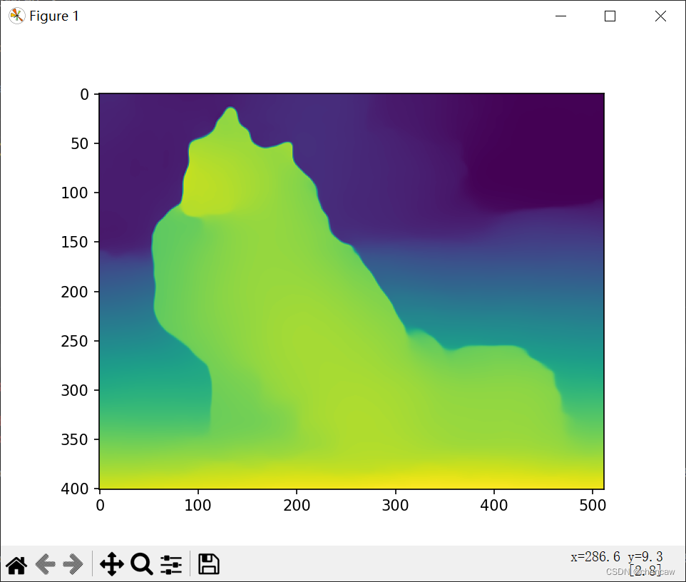
#(6)Show result
plt.imshow(output)
plt.show()
# plt.show()(2)测试结果
7、单目摄像头深度图完整例子
(1)完整代码
import torch
import matplotlib.pyplot as plt
import cv2
import numpy as np
import time

##直接将D:/RGBD_CAMERA/mis/MiDaS-master/hubconf.py中的transforms拿来使用
def transforms():
    import cv2
    from torchvision.transforms import Compose
    from midas.transforms import Resize, NormalizeImage, PrepareForNet
    from midas import transforms

    transforms.default_transform = Compose(
        [
            lambda img: {"image": img / 255.0},
            Resize(
                384,
                384,
                resize_target=None,
                keep_aspect_ratio=True,
                ensure_multiple_of=32,
                resize_method="upper_bound",
                image_interpolation_method=cv2.INTER_CUBIC,
            ),
            NormalizeImage(mean=[0.485, 0.456, 0.406], std=[0.229, 0.224, 0.225]),
            PrepareForNet(),
            lambda sample: torch.from_numpy(sample["image"]).unsqueeze(0),
        ]
    )

    transforms.small_transform = Compose(
        [
            lambda img: {"image": img / 255.0},
            Resize(
                256,
                256,
                resize_target=None,
                keep_aspect_ratio=True,
                ensure_multiple_of=32,
                resize_method="upper_bound",
                image_interpolation_method=cv2.INTER_CUBIC,
            ),
            NormalizeImage(mean=[0.485, 0.456, 0.406], std=[0.229, 0.224, 0.225]),
            PrepareForNet(),
            lambda sample: torch.from_numpy(sample["image"]).unsqueeze(0),
        ]
    )

    transforms.dpt_transform = Compose(
        [
            lambda img: {"image": img / 255.0},
            Resize(
                384,
                384,
                resize_target=None,
                keep_aspect_ratio=True,
                ensure_multiple_of=32,
                resize_method="minimal",
                image_interpolation_method=cv2.INTER_CUBIC,
            ),
            NormalizeImage(mean=[0.5, 0.5, 0.5], std=[0.5, 0.5, 0.5]),
            PrepareForNet(),
            lambda sample: torch.from_numpy(sample["image"]).unsqueeze(0),
        ]
    )

    return transforms


# (一)方法一、使用torch.hub或者从官网下载
# https://github.com/isl-org/MiDaS#Accuracy
# model_type = "DPT_Large"     # MiDaS v3 - Large     (highest accuracy, slowest inference speed)
# #model_type = "DPT_Hybrid"   # MiDaS v3 - Hybrid    (medium accuracy, medium inference speed)
# #model_type = "MiDaS_small"  # MiDaS v2.1 - Small   (lowest accuracy, highest inference speed)
# midas = torch.hub.load("intel-isl/MiDaS", model_type)

# (二)方法二、下载本地后直接加载
# (1)Load a model
model_type = "DPT_Large"
# midas = torch.hub.load('intel-isl/MiDaS', path='D:/BaiduNetdiskDownload/dpt_large-midas-2f21e586.pt', source='local',model =model_type )
# midas = torch.hub.load('D:/RGBD_CAMERA/mis/MiDaS-master', path='D:/BaiduNetdiskDownload/dpt_large-midas-2f21e586.pt', source='local',model =model_type,force_reload = False )
midas = torch.hub.load('D:/RGBD_CAMERA/mis/MiDaS-master', source='local',model =model_type,force_reload = False )

#(2)Move model to GPU if available
device = torch.device("cuda") if torch.cuda.is_available() else torch.device("cpu")
midas.to(device)
midas.eval()

#(3)Load transforms to resize and normalize the image for large or small model
# midas_transforms = torch.hub.load("intel-isl/MiDaS", "transforms")
midas_transforms = transforms()

if model_type == "DPT_Large" or model_type == "DPT_Hybrid":
    transform = midas_transforms.dpt_transform
else:
    transform = midas_transforms.small_transform

print("chen0")
#(4)Load image and apply transforms
filename = 'D:/RGBD_CAMERA/python_3d_process/dog.jpg'
img = cv2.imread(filename)
img = cv2.cvtColor(img, cv2.COLOR_BGR2RGB)
print("chen1")
input_batch = transform(img).to(device)

#(5)Predict and resize to original resolution
with torch.no_grad():
    prediction = midas(input_batch)

    prediction = torch.nn.functional.interpolate(
        prediction.unsqueeze(1),
        size=img.shape[:2],
        mode="bicubic",
        align_corners=False,
    ).squeeze()

output = prediction.cpu().numpy()
print(output.shape)
print("chen2")
#(6)Show result
plt.imshow(output)
plt.show()
cv2.waitKey(0)

##下面是通过摄像头捕获图片,而后三维重建相关的
######三维重建
Q = np.array(([1.0, 0.0, 0.0, -160.0],
              [0.0, 1.0, 0.0, -120.0],
              [0.0, 0.0, 0.0, 350.0],
              [0.0, 0.0, 1.0/90.0, 0.0]),dtype=np.float32)


# Open up the video capture from a webcam
cap = cv2.VideoCapture(1)
print("chencap")

while cap.isOpened():

    success, img = cap.read()

    start = time.time()
    cv2.imshow("origin_pic",img)

    img = cv2.cvtColor(img, cv2.COLOR_BGR2RGB)

    # Apply input transforms
    input_batch = transform(img).to(device)

    # Prediction and resize to original resolution
    with torch.no_grad():
        prediction = midas(input_batch)

        prediction = torch.nn.functional.interpolate(
            prediction.unsqueeze(1),
            size=img.shape[:2],
            mode="bicubic",
            align_corners=False,
        ).squeeze()

    depth_map = prediction.cpu().numpy()

    depth_map = cv2.normalize(depth_map, None, 0, 1, norm_type=cv2.NORM_MINMAX, dtype=cv2.CV_32F)

    #Reproject points into 3D
    points_3D = cv2.reprojectImageTo3D(depth_map, Q, handleMissingValues=False)


    #Get rid of points with value 0 (i.e no depth)
    mask_map = depth_map > 0.4

    #Mask colors and points.
    output_points = points_3D[mask_map]
    output_colors = img[mask_map]

    end = time.time()
    totalTime = end - start

    fps = 1 / totalTime

    img = cv2.cvtColor(img, cv2.COLOR_RGB2BGR)


    depth_map = (depth_map*255).astype(np.uint8)
    depth_map = cv2.applyColorMap(depth_map , cv2.COLORMAP_MAGMA)


    cv2.putText(img, f'FPS: {int(fps)}', (20,70), cv2.FONT_HERSHEY_SIMPLEX, 1.5, (0,255,0), 2)
    cv2.imshow('Image', img)
    cv2.imshow('Depth Map', depth_map)

    if cv2.waitKey(5) & 0xFF == 27:
        break


# --------------------- Create The Point Clouds ----------------------------------------

#Function to create point cloud file
def create_output(vertices, colors, filename):
	colors = colors.reshape(-1,3)
	vertices = np.hstack([vertices.reshape(-1,3),colors])

	ply_header = '''ply
		format ascii 1.0
		element vertex %(vert_num)d
		property float x
		property float y
		property float z
		property uchar red
		property uchar green
		property uchar blue
		end_header
		'''
	with open(filename, 'w') as f:
		f.write(ply_header %dict(vert_num=len(vertices)))
		np.savetxt(f,vertices,'%f %f %f %d %d %d')


output_file = 'pointCloudDeepLearning.ply'
#Generate point cloud
create_output(output_points, output_colors, output_file)

cap.release()
cv2.destroyAllWindows()
(2)显示的代码
# pip install -i https://pypi.tuna.tsinghua.edu.cn/simple open3d
# pip install open3d -i https://pypi.tuna.tsinghua.edu.cn/simple
#xachen 显示可以了,20221128


import open3d as o3d
import numpy as np

##--方法(1)去除Nan------------------
# path = "D:/RGBD_CAMERA/python_3d_process/1_hezi.pcd"
# pcd = o3d.io.read_point_cloud(path)  # path为文件路径
# pcd_new = o3d.geometry.PointCloud.remove_non_finite_points(
#                         pcd, remove_nan = True, remove_infinite = False)
# o3d.visualization.draw_geometries([pcd_new])


##--方法(2)去除Nan------------------
# path = "D:/RGBD_CAMERA/python_3d_process/1_hezi.pcd"
# path = "D:/RGBD_CAMERA/python_3d_process/chenmobile.pcd"
path = "D:/RGBD_CAMERA/python_3d_process/pointCloudDeepLearning.ply"
pcd = o3d.io.read_point_cloud(path)  # path为文件路径
# res = pcd.remove_non_finite_points(True, True)#剔除无效值
pcd = pcd.remove_non_finite_points(True, False)#剔除无效值
o3d.visualization.draw_geometries([pcd],
                                      window_name="窗口名字测试",
                                      point_show_normal=False,
                                      width=800,  # 窗口宽度
                                      height=600)  # 窗口高度
完结撒花
------------------------------------------------------------
-------------------------------------------------------------
#注意:下面的教程和描述先不要管,待完善!
------------------------------------------
???
5.2大佬的测试教程
(1)测试代码
import cv2
import torch
import time
import numpy as np

#该文件参考地址
# https://github.com/niconielsen32/ComputerVision/blob/master/depthToPointCloud.py

# model = torch.hub.load('ultralytics/yolov5', 'custom', path='path/to/best.pt')

# Q matrix - Camera parameters - Can also be found using stereoRectify
Q = np.array(([1.0, 0.0, 0.0, -160.0],
              [0.0, 1.0, 0.0, -120.0],
              [0.0, 0.0, 0.0, 350.0],
              [0.0, 0.0, 1.0/90.0, 0.0]),dtype=np.float32)

# Load a MiDas model for depth estimation
model_type = "DPT_Large"     # MiDaS v3 - Large     (highest accuracy, slowest inference speed)
#model_type = "DPT_Hybrid"   # MiDaS v3 - Hybrid    (medium accuracy, medium inference speed)
#model_type = "MiDaS_small"  # MiDaS v2.1 - Small   (lowest accuracy, highest inference speed)

midas = torch.hub.load("intel-isl/MiDaS", model_type)

# Move model to GPU if available
device = torch.device("cuda") if torch.cuda.is_available() else torch.device("cpu")
midas.to(device)
midas.eval()

# Load transforms to resize and normalize the image
midas_transforms = torch.hub.load("intel-isl/MiDaS", "transforms")

if model_type == "DPT_Large" or model_type == "DPT_Hybrid":
    transform = midas_transforms.dpt_transform
else:
    transform = midas_transforms.small_transform


# Open up the video capture from a webcam
cap = cv2.VideoCapture(2)

while cap.isOpened():

    success, img = cap.read()

    start = time.time()

    img = cv2.cvtColor(img, cv2.COLOR_BGR2RGB)

    # Apply input transforms
    input_batch = transform(img).to(device)

    # Prediction and resize to original resolution
    with torch.no_grad():
        prediction = midas(input_batch)

        prediction = torch.nn.functional.interpolate(
            prediction.unsqueeze(1),
            size=img.shape[:2],
            mode="bicubic",
            align_corners=False,
        ).squeeze()

    depth_map = prediction.cpu().numpy()

    depth_map = cv2.normalize(depth_map, None, 0, 1, norm_type=cv2.NORM_MINMAX, dtype=cv2.CV_32F)

    #Reproject points into 3D
    points_3D = cv2.reprojectImageTo3D(depth_map, Q, handleMissingValues=False)


    #Get rid of points with value 0 (i.e no depth)
    mask_map = depth_map > 0.4

    #Mask colors and points.
    output_points = points_3D[mask_map]
    output_colors = img[mask_map]

    end = time.time()
    totalTime = end - start

    fps = 1 / totalTime

    img = cv2.cvtColor(img, cv2.COLOR_RGB2BGR)


    depth_map = (depth_map*255).astype(np.uint8)
    depth_map = cv2.applyColorMap(depth_map , cv2.COLORMAP_MAGMA)


    cv2.putText(img, f'FPS: {int(fps)}', (20,70), cv2.FONT_HERSHEY_SIMPLEX, 1.5, (0,255,0), 2)
    cv2.imshow('Image', img)
    cv2.imshow('Depth Map', depth_map)

    if cv2.waitKey(5) & 0xFF == 27:
        break


# --------------------- Create The Point Clouds ----------------------------------------

#Function to create point cloud file
def create_output(vertices, colors, filename):
	colors = colors.reshape(-1,3)
	vertices = np.hstack([vertices.reshape(-1,3),colors])

	ply_header = '''ply
		format ascii 1.0
		element vertex %(vert_num)d
		property float x
		property float y
		property float z
		property uchar red
		property uchar green
		property uchar blue
		end_header
		'''
	with open(filename, 'w') as f:
		f.write(ply_header %dict(vert_num=len(vertices)))
		np.savetxt(f,vertices,'%f %f %f %d %d %d')


output_file = 'pointCloudDeepLearning.ply'
#Generate point cloud
create_output(output_points, output_colors, output_file)

cap.release()
cv2.destroyAllWindows()
?????
测试方法
2.1下载模型
 (2)真是一个big的模型啊
2.2 转为onnx
实际上转完后opencv无法调研
3.使用pytorch hub的方法直接调用


 749
749


 到【灌水乐园】发言


