


一、 Adaboost的基本原理
-
集成学习思想:Adaboost是一种集成学习方法,通过组合多个弱学习器(如浅层决策树)来构建一个强学习器。每个弱学习器专注于前一个学习器预测错误的样本,逐步提高整体模型的预测精度。
-
加权训练机制:算法为每个训练样本分配权重,初始权重相同。每次迭代中,训练一个弱学习器,根据其预测错误率调整样本权重——增加错误预测样本的权重,减少正确预测样本的权重。这样后续学习器会更关注难以预测的样本。
-
加权投票预测:每个弱学习器根据其训练准确率被赋予一个权重,准确率越高,权重越大。最终预测结果是所有弱学习器预测值的加权组合。
二、时间序列适应的特殊性
-
序列依赖性处理:虽然Adaboost本身不考虑时间序列的自相关性,但通过特征工程(如创建滞后变量、移动平均等时间相关特征)将时间依赖性转化为特征,使模型能够学习时间模式。
-
非线性关系捕捉:Adaboost通过组合多个决策树,能够捕捉时间序列中的非线性关系和复杂模式,这对于金融、经济等具有非线性特征的时间序列特别重要。
-
自适应调整能力:由于时间序列可能随时间变化(概念漂移),Adaboost的迭代加权机制使其能够自适应调整,对新的数据模式保持敏感。
-
误差纠正机制:在时间序列预测中,某些时期(如市场波动期)可能难以预测。Adaboost通过增加这些困难时期的样本权重,让后续学习器更专注学习这些模式。
四 与其他时间序列预测算法的对比优势
三、与其他算法相比,Adaboost的优势
相比传统统计方法(ARIMA、指数平滑等):
-
无需严格假设:传统方法通常需要序列平稳性、线性关系等假设,而Adaboost不需要这些严格假设,适用范围更广。
-
非线性处理能力:能够捕捉复杂的非线性关系,而传统方法主要处理线性关系。
-
多变量整合:更容易整合多变量信息,而传统单变量方法只能处理自身历史信息。
相比单一机器学习模型(如单一决策树、SVM等):
-
降低过拟合风险:通过集成多个弱学习器,减少了单一复杂模型过拟合的风险,尤其适合噪声较多的时间序列数据。
-
提升泛化能力:加权投票机制使模型更稳健,对异常值和噪声有更好的抵抗力。
-
自动特征重要性:可以评估不同时间滞后特征的重要性,帮助理解时间序列的关键影响因素。
相比其他集成方法(如随机森林):
-
关注困难样本:Adaboost特别关注之前预测错误的样本,可能对时间序列中的转折点、突变点更敏感。
-
序列训练优势:Adaboost的序列训练方式可能更适合时间序列的顺序特性。
-
模型解释性:虽然都是集成方法,但Adaboost的加权机制提供了额外的模型解释维度。
相比深度学习模型(LSTM、GRU等):
-
计算效率高:训练和预测速度通常比深度学习方法快,不需要GPU支持。
-
小数据表现好:在小样本时间序列数据上表现更稳定,而深度学习方法通常需要大量数据。
-
超参数调整简单:需要调整的超参数较少,更易于使用和调优。
-
可解释性更强:决策树基础的Adaboost比神经网络更容易理解和解释。
优势小节
-
处理不平稳序列:对非平稳时间序列有较好的适应性,不需要预先进行复杂的平稳化处理。
-
多尺度特征学习:通过组合不同深度的决策树,可以同时学习时间序列的长期趋势和短期波动。
-
鲁棒性:对异常值、缺失值和噪声数据具有较好的鲁棒性。
-
灵活的特征组合:可以自然地结合时间序列特征(滞后值、移动统计量)与其他相关特征(如外部经济指标)。
-
自适应权重调整:能够根据预测误差动态调整不同时间段的关注度,对变化的时间序列模式更敏感。
四、应用实例
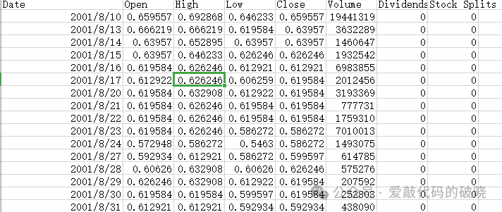
1.数据准备
2.导入第三方库
import numpy as np
import pandas as pd
import matplotlib.pyplot as plt
import seaborn as sns
from sklearn.model_selection import train_test_split
from sklearn.ensemble import AdaBoostRegressor
from sklearn.tree import DecisionTreeRegressor
from sklearn.metrics import mean_squared_error, mean_absolute_error, r2_score
import joblib
import warnings
import argparse
import os
import sys
from matplotlib.colors import LinearSegmentedColormap
from scipy.stats import gaussian_kde

warnings.filterwarnings('ignore')
3.绘图设置
# 设置中文字体和样式
plt.rcParams['font.sans-serif'] = ['SimHei', 'Microsoft YaHei', 'DejaVu Sans']
plt.rcParams['axes.unicode_minus'] = False
# sns.set_style("whitegrid")
4.Adaboost模型构
def __init__(self, n_estimators=100, learning_rate=0.1, max_depth=3):
        self.n_estimators = n_estimators
        self.learning_rate = learning_rate
        self.max_depth = max_depth
        self.model = None
        self.feature_names = None
        self.window_size = 10

    def create_features(self, series, window_size=10):
        """创建时间序列特征"""
        df = pd.DataFrame(series, columns=['Open'])

        # 滞后特征
        for i in range(1, window_size + 1):
            df[f'lag_{i}'] = df['Open'].shift(i)

        # 移动平均特征
        df['rolling_mean_5'] = df['Open'].rolling(window=5).mean().shift(1)
        df['rolling_std_5'] = df['Open'].rolling(window=5).std().shift(1)

        # 目标变量(下一时刻的Open值)
        df['target'] = df['Open'].shift(-1)

        # 删除含有NaN的行
        df = df.dropna()

        # 特征和标签
        X = df.drop(['target', 'Open'], axis=1)
        y = df['target']

        return X, y
5.训练Adaboost模型
def train(self, data_path, window_size=10, test_size=0.2, random_state=42):
        """训练模型"""
        print("正在读取数据...")
        # 读取数据
        df = pd.read_csv(data_path, parse_dates=['Date'])

        print(f"数据形状: {df.shape}")
        print(f"数据列名: {df.columns.tolist()}")

        # 使用Open列
        series = df['Open'].values
        self.window_size = window_size

        # 创建特征
        print("创建时间序列特征...")
        X, y = self.create_features(df['Open'], window_size)
        self.feature_names = X.columns.tolist()

        # 划分训练集和测试集
        print(f"划分训练集和测试集 ({1-test_size}:{test_size})...")
        X_train, X_test, y_train, y_test = train_test_split(
            X, y, test_size=test_size, shuffle=False, random_state=random_state
        )

        print(f"训练集形状: {X_train.shape}, 测试集形状: {X_test.shape}")

        # 创建并训练AdaBoost模型
        print("训练AdaBoost回归模型...")
        base_estimator = DecisionTreeRegressor(
            max_depth=self.max_depth,
            random_state=random_state
        )

        self.model = AdaBoostRegressor(
            base_estimator=base_estimator,
            n_estimators=self.n_estimators,
            learning_rate=self.learning_rate,
            random_state=random_state
        )

        self.model.fit(X_train, y_train)

        # 预测
        y_train_pred = self.model.predict(X_train)
        y_test_pred = self.model.predict(X_test)

        # 评估指标
        print("\n" + "="*50)
        print("模型评估结果:")
        print("="*50)

        train_metrics = self.calculate_metrics(y_train, y_train_pred, "训练集")
        test_metrics = self.calculate_metrics(y_test, y_test_pred, "测试集")

        # 保存结果
        self.X_train, self.X_test = X_train, X_test
        self.y_train, self.y_test = y_train, y_test
        self.y_train_pred, self.y_test_pred = y_train_pred, y_test_pred

        # 获取训练和测试的日期索引(用于绘图)
        train_indices = df.index[-len(y):][:len(y_train)]
        test_indices = df.index[-len(y):][len(y_train):len(y_train)+len(y_test)]

        self.train_dates = df['Date'].iloc[train_indices].values
        self.test_dates = df['Date'].iloc[test_indices].values
        self.original_dates = df['Date'].iloc[-len(y):].values
        self.full_y_true = y.values
        self.full_y_pred = np.concatenate([y_train_pred, y_test_pred])

        return {
            'train_metrics': train_metrics,
            'test_metrics': test_metrics,
            'model': self.model,
            'feature_names': self.feature_names,
            'window_size': self.window_size
        }
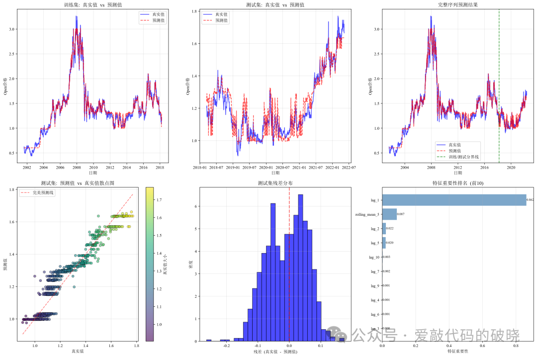
6.Adaboost模型预测
def plot_predictions(self):
"""绘制预测结果"""
if self.model is None:
print("请先训练模型!")
return
fig, axes = plt.subplots(2, 3, figsize=(18, 12))
# 1. 训练集预测曲线
ax1 = axes[0, 0]
ax1.plot(self.train_dates, self.y_train, 'b-', label='真实值', alpha=0.7, linewidth=1.5)
ax1.plot(self.train_dates, self.y_train_pred, 'r--', label='预测值', alpha=0.7, linewidth=1.5)
ax1.set_title('训练集: 真实值 vs 预测值', fontweight='bold')
ax1.set_xlabel('日期')
ax1.set_ylabel('Open价格')
ax1.legend(loc='best')
ax1.grid(True, alpha=0.3)
# 2. 测试集预测曲线
ax2 = axes[0, 1]
ax2.plot(self.test_dates, self.y_test, 'b-', label='真实值', alpha=0.7, linewidth=1.5)
ax2.plot(self.test_dates, self.y_test_pred, 'r--', label='预测值', alpha=0.7, linewidth=1.5)
ax2.set_title('测试集: 真实值 vs 预测值', fontweight='bold')
ax2.set_xlabel('日期')
ax2.set_ylabel('Open价格')
ax2.legend(loc='best')
ax2.grid(True, alpha=0.3)
# 3. 完整序列预测曲线
ax3 = axes[0, 2]
all_dates = np.concatenate([self.train_dates, self.test_dates])
all_y_true = np.concatenate([self.y_train, self.y_test])
all_y_pred = np.concatenate([self.y_train_pred, self.y_test_pred])
ax3.plot(all_dates, all_y_true, 'b-', label='真实值', alpha=0.7, linewidth=1.5)
ax3.plot(all_dates, all_y_pred, 'r--', label='预测值', alpha=0.7, linewidth=1.5)
ax3.axvline(x=self.test_dates[0], color='g', linestyle='--', alpha=0.7,
linewidth=1.5, label='训练/测试分界线')
ax3.set_title('完整序列预测结果', fontweight='bold')
ax3.set_xlabel('日期')
ax3.set_ylabel('Open价格')
ax3.legend(loc='best')
ax3.grid(True, alpha=0.3)
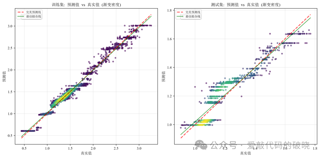
# 4. 预测值与真实值散点图(带密度)
ax4 = axes[1, 0]
scatter = ax4.scatter(self.y_test, self.y_test_pred, c=self.y_test,
cmap='viridis', alpha=0.6, edgecolors='k', linewidth=0.5)
ax4.plot([self.y_test.min(), self.y_test.max()],
[self.y_test.min(), self.y_test.max()],
'r--', alpha=0.5, label='完美预测线')
ax4.set_xlabel('真实值')
ax4.set_ylabel('预测值')
ax4.set_title('测试集: 预测值 vs 真实值散点图', fontweight='bold')
ax4.legend(loc='best')
ax4.grid(True, alpha=0.3)
plt.colorbar(scatter, ax=ax4, label='真实值大小')
# 5. 残差分布图
ax5 = axes[1, 1]
residuals = self.y_test - self.y_test_pred
ax5.hist(residuals, bins=30, density=True, alpha=0.7, color='blue', edgecolor='black')
ax5.axvline(x=0, color='red', linestyle='--', alpha=0.5, linewidth=2)
ax5.set_xlabel('残差 (真实值 - 预测值)')
ax5.set_ylabel('密度')
ax5.set_title('测试集残差分布', fontweight='bold')
ax5.grid(True, alpha=0.3)
# 6. 特征重要性
ax6 = axes[1, 2]
if hasattr(self.model, 'feature_importances_'):
feature_importance = self.model.feature_importances_
features = self.feature_names if self.feature_names else [f'特征_{i}' for i in range(len(feature_importance))]
# 只显示前10个最重要的特征
if len(feature_importance) > 10:
indices = np.argsort(feature_importance)[-10:]
feature_importance = feature_importance[indices]
features = [features[i] for i in indices]
bars = ax6.barh(range(len(feature_importance)), feature_importance, alpha=0.7, color='steelblue')
ax6.set_yticks(range(len(feature_importance)))
ax6.set_yticklabels(features, fontsize=9)
ax6.set_xlabel('特征重要性')
ax6.set_title('特征重要性排名 (前10)', fontweight='bold')
ax6.grid(True, alpha=0.3, axis='x')
# 添加数值标签
for i, bar in enumerate(bars):
width = bar.get_width()
ax6.text(width + 0.001, bar.get_y() + bar.get_height()/2,
f'{width:.3f}', ha='left', va='center', fontsize=8)
plt.tight_layout()
plt.savefig('adaBoost_predictions.png', dpi=300, bbox_inches='tight')
plt.show()
7.Adaboost模型评价
def calculate_metrics(self, y_true, y_pred, dataset_name):
        """计算评估指标"""
        mse = mean_squared_error(y_true, y_pred)
        rmse = np.sqrt(mse)
        mae = mean_absolute_error(y_true, y_pred)
        r2 = r2_score(y_true, y_pred)
        mape = np.mean(np.abs((y_true - y_pred) / y_true)) * 100

        metrics = {
            'MSE': mse,
            'RMSE': rmse,
            'MAE': mae,
            'R²': r2,
            'MAPE': mape
        }

        print(f"\n{dataset_name}评估指标:")
        print(f"  MSE: {mse:.4f}")
        print(f"  RMSE: {rmse:.4f}")
        print(f"  MAE: {mae:.4f}")
        print(f"  R²: {r2:.4f}")
        print(f"  MAPE: {mape:.2f}%")
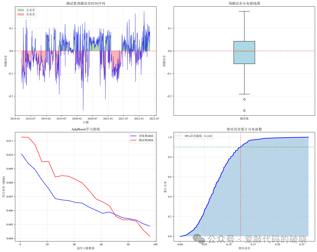
8.绘图
def plot_additional_charts(self):
    """绘制额外的分析图表"""
    fig, axes = plt.subplots(2, 2, figsize=(15, 12))

    # 1. 误差随时间变化
    ax1 = axes[0, 0]
    test_errors = self.y_test - self.y_test_pred
    ax1.plot(self.test_dates, test_errors, 'b-', alpha=0.7, linewidth=1)
    ax1.axhline(y=0, color='r', linestyle='--', alpha=0.5, linewidth=1.5)
    ax1.fill_between(self.test_dates, 0, test_errors, where=(test_errors>0),
                    color='green', alpha=0.3, label='正误差')
    ax1.fill_between(self.test_dates, 0, test_errors, where=(test_errors<0),
                    color='red', alpha=0.3, label='负误差')
    ax1.set_xlabel('日期')
    ax1.set_ylabel('预测误差')
    ax1.set_title('测试集预测误差时间序列', fontweight='bold')
    ax1.legend(loc='best')
    ax1.grid(True, alpha=0.3)

    # 2. 预测误差箱线图
    ax2 = axes[0, 1]
    bp = ax2.boxplot(test_errors, patch_artist=True)
    bp['boxes'][0].set_facecolor('lightblue')
    ax2.axhline(y=0, color='r', linestyle='--', alpha=0.5, linewidth=1.5)
    ax2.set_ylabel('预测误差')
    ax2.set_title('预测误差分布箱线图', fontweight='bold')
    ax2.grid(True, alpha=0.3)
    ax2.set_xticks([1])
    ax2.set_xticklabels(['测试集'])

    # 3. 模型学习曲线(误差随弱学习器数量变化)
    ax3 = axes[1, 0]
    train_errors = []
    test_errors_list = []

    # 计算不同阶段模型性能
    for n in range(1, self.model.n_estimators + 1, max(1, self.model.n_estimators // 20)):
        model_partial = AdaBoostRegressor(
            base_estimator=DecisionTreeRegressor(max_depth=self.max_depth),
            n_estimators=n,
            learning_rate=self.learning_rate,
            random_state=42
        )
        model_partial.fit(self.X_train, self.y_train)

        train_pred = model_partial.predict(self.X_train)
        test_pred = model_partial.predict(self.X_test)

        train_errors.append(mean_squared_error(self.y_train, train_pred))
        test_errors_list.append(mean_squared_error(self.y_test, test_pred))

    iterations = range(1, self.model.n_estimators + 1, max(1, self.model.n_estimators // 20))
    ax3.plot(iterations, train_errors, 'b-', label='训练集MSE', linewidth=1.5)
    ax3.plot(iterations, test_errors_list, 'r-', label='测试集MSE', linewidth=1.5)
    ax3.set_xlabel('弱学习器数量')
    ax3.set_ylabel('均方误差 (MSE)')
    ax3.set_title('AdaBoost学习曲线', fontweight='bold')
    ax3.legend(loc='best')
    ax3.grid(True, alpha=0.3)

    # 4. 累计误差分布图
    ax4 = axes[1, 1]
    sorted_errors = np.sort(np.abs(test_errors))
    cumulative = np.cumsum(sorted_errors) / np.sum(sorted_errors)
    ax4.plot(sorted_errors, cumulative, 'b-', linewidth=2)
    ax4.fill_between(sorted_errors, 0, cumulative, alpha=0.3)

    # 标记90%误差阈值
    idx_90 = np.where(cumulative >= 0.9)[0][0] if len(cumulative) > 0 else 0
    if len(sorted_errors) > idx_90:
        ax4.axvline(x=sorted_errors[idx_90], color='r', linestyle='--', alpha=0.5,
                   label=f'90%误差阈值: {sorted_errors[idx_90]:.4f}')
        ax4.axhline(y=0.9, color='g', linestyle='--', alpha=0.5)

    ax4.set_xlabel('绝对误差')
    ax4.set_ylabel('累计分布')
    ax4.set_title('绝对误差累计分布函数', fontweight='bold')
    ax4.legend(loc='best')
    ax4.grid(True, alpha=0.3)

    plt.tight_layout()
    plt.savefig('adaBoost_analysis.png', dpi=300, bbox_inches='tight')
    plt.show()
以下是程序运行的结果:
五、总结
-
总结等复杂度的非线性模式时,Adaboost通常表现良好。
-
需要可解释性的场景:相比黑箱模型,Adaboost提供了一定程度的可解释性。
-
计算资源有限的环境:在计算资源受限的情况下,Adaboost是深度学习的良好替代方案。
-
多变量时间序列预测:当需要同时考虑多个相关时间序列或外部因素时。
需要注意的是,Adaboost并非在所有时间序列预测任务中都表现最佳。对于具有强长期依赖性的序列,或需要捕捉复杂时间动态的序列,LSTM等深度学习方法可能更合适。但对于许多实际应用场景,特别是那些需要平衡准确性、计算效率和可解释性的场景,Adaboost是一个非常有竞争力的选择。


 2584
2584

 被折叠的 条评论
为什么被折叠?
被折叠的 条评论
为什么被折叠?
 到【灌水乐园】发言


