


文章较长,示例代码在第三个部分,如需要数据及源码,关注微信公众号【爱敲代码的破晓】,后台私信【20251228】
一、基本概念
LSTM是一种特殊的循环神经网络(RNN),由Sepp Hochreiter和Jürgen Schmidhuber于1997年提出,专门用于解决传统RNN在处理长序列数据时遇到的梯度消失/爆炸问题。
二、LSTM适用场景
-
✅ 长期依赖的时间序列(气象、股价、生理信号)
-
✅ 多变量时间序列(多个相关变量)
-
✅ 非平稳、非线性序列
-
✅ 需要捕捉复杂模式的任务
三、LSTM适用场景
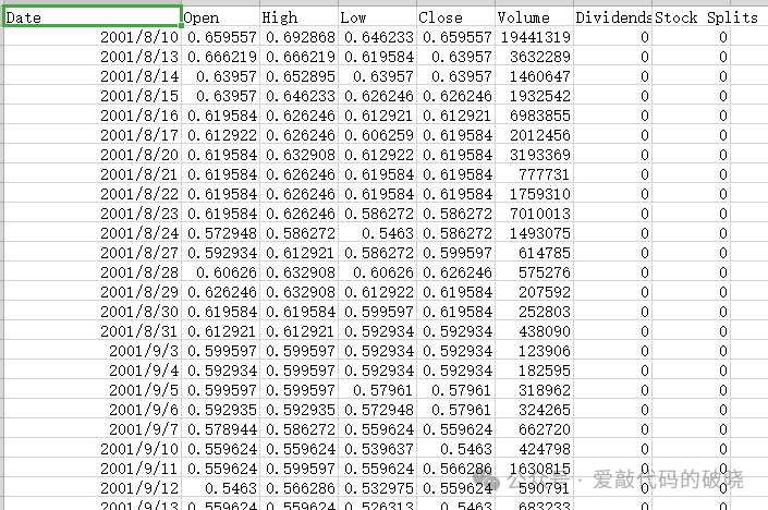
1.数据准备
2.导入第三方库
import numpy as np
import pandas as pd
import matplotlib.pyplot as plt
from sklearn.preprocessing import MinMaxScaler
from sklearn.model_selection import train_test_split
from tensorflow.keras.models import Sequential, load_model
from tensorflow.keras.layers import LSTM, Dense, Dropout
from tensorflow.keras.callbacks import EarlyStopping, ModelCheckpoint
import joblib
import os
import warnings
warnings.filterwarnings('ignore')
3.设置随机种子
# 设置随机种子以确保结果可重现
np.random.seed(42)
4.导入数据模块
def load_and_preprocess_data(filepath):
    """
    加载和预处理数据
    """
    # 读取CSV文件
    df = pd.read_csv(filepath, parse_dates=['Date'])

    print(f"数据形状: {df.shape}")
    print(f"数据列名: {df.columns.tolist()}")
    print(f"数据时间范围: {df['Date'].min()} 到 {df['Date'].max()}")
    print(f"数据统计信息:")
    print(df[['Open']].describe())

    # 使用Open列作为目标变量
    data = df[['Open']].values

    # 数据归一化
    scaler = MinMaxScaler(feature_range=(0, 1))
    data_scaled = scaler.fit_transform(data)

    return data_scaled, df, scaler
5.构建LSTM框架模块
def build_lstm_model(input_shape):
    """
    构建LSTM模型
    """
    model = Sequential([
        LSTM(units=50, return_sequences=True, input_shape=input_shape),
        Dropout(0.2),
        LSTM(units=50, return_sequences=True),
        Dropout(0.2),
        LSTM(units=50),
        Dropout(0.2),
        Dense(units=1)
    ])

    model.compile(optimizer='adam', loss='mean_squared_error')
    model.summary()

    return model
6.预测评估模块
def evaluate_predictions(y_true, y_pred, set_name="测试集"):
    """
    评估预测结果
    """
    # 计算评估指标
    mse = mean_squared_error(y_true, y_pred)
    rmse = np.sqrt(mse)
    mae = mean_absolute_error(y_true, y_pred)
    r2 = r2_score(y_true, y_pred)

    # 计算平均绝对百分比误差 (MAPE)
    mape = np.mean(np.abs((y_true - y_pred) / y_true)) * 100

    print(f"\n{set_name}评估指标:")
    print(f"均方误差 (MSE): {mse:.4f}")
    print(f"均方根误差 (RMSE): {rmse:.4f}")
    print(f"平均绝对误差 (MAE): {mae:.4f}")
    print(f"R²分数: {r2:.4f}")
    print(f"平均绝对百分比误差 (MAPE): {mape:.2f}%")

    return {
        'MSE': mse,
        'RMSE': rmse,
        'MAE': mae,
        'R2': r2,
        'MAPE': mape
    }
7.绘制图件模块
def plot_predictions(df, train_predict, y_train_actual, test_predict, y_test_actual,
look_back, scaler, train_metrics, test_metrics):
"""
绘制多种预测结果图表
"""
# 创建完整的图表
fig = plt.figure(figsize=(20, 16))
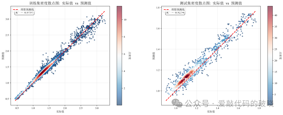
# 1. 训练集密度散点图
ax1 = plt.subplot(3, 3, 1)
plot_density_scatter(y_train_actual, train_predict, "训练集", ax1)
# 2. 测试集密度散点图
ax2 = plt.subplot(3, 3, 2)
plot_density_scatter(y_test_actual, test_predict, "测试集", ax2)
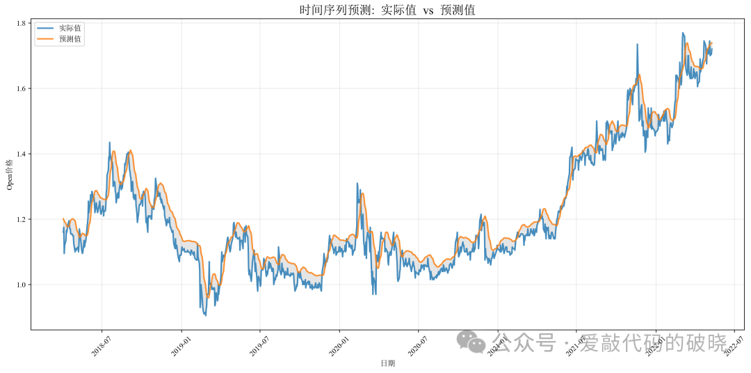
# 3. 训练集和测试集预测曲线对比
ax3 = plt.subplot(3, 3, 3)
# 创建时间索引
train_size = len(train_predict)
train_dates = df['Date'].iloc[look_back+1:look_back+1+train_size]
test_dates = df['Date'].iloc[look_back+1+train_size:look_back+1+train_size+len(test_predict)]
ax3.plot(train_dates, y_train_actual, label='训练集实际值', linewidth=1.5, alpha=0.7)
ax3.plot(train_dates, train_predict, label='训练集预测值', linewidth=1.5, alpha=0.7)
ax3.plot(test_dates, y_test_actual, label='测试集实际值', linewidth=1.5, alpha=0.7)
ax3.plot(test_dates, test_predict, label='测试集预测值', linewidth=1.5, alpha=0.7)
# 添加垂直线分隔训练集和测试集
if len(train_dates) > 0 and len(test_dates) > 0:
ax3.axvline(x=separation_date, color='black', linestyle='--', linewidth=1, alpha=0.5)
ax3.text(separation_date, ax3.get_ylim()[1]*0.95, '测试集开始',
rotation=90, verticalalignment='top', fontsize=10)
ax3.set_title('训练集和测试集预测曲线对比', fontsize=14, fontweight='bold')
ax3.set_xlabel('日期')
ax3.set_ylabel('Open价格')
ax3.legend(loc='upper left')
ax3.grid(True, alpha=0.3)
plt.setp(ax3.xaxis.get_majorticklabels(), rotation=45)
# 4. 训练集预测误差分布
ax4 = plt.subplot(3, 3, 4)
train_errors = y_train_actual.flatten() - train_predict.flatten()
ax4.hist(train_errors, bins=50, edgecolor='black', alpha=0.7, color='skyblue', density=True)
ax4.axvline(x=0, color='r', linestyle='--', linewidth=2)
ax4.set_title('训练集预测误差分布', fontsize=14, fontweight='bold')
ax4.set_xlabel('预测误差')
ax4.set_ylabel('密度')
ax4.grid(True, alpha=0.3)
# 5. 测试集预测误差分布
ax5 = plt.subplot(3, 3, 5)
test_errors = y_test_actual.flatten() - test_predict.flatten()
ax5.hist(test_errors, bins=50, edgecolor='black', alpha=0.7, color='lightcoral', density=True)
ax5.axvline(x=0, color='r', linestyle='--', linewidth=2)
ax5.set_title('测试集预测误差分布', fontsize=14, fontweight='bold')
ax5.set_xlabel('预测误差')
ax5.set_ylabel('密度')
ax5.grid(True, alpha=0.3)
# 6. 相对误差百分比对比
ax6 = plt.subplot(3, 3, 6)
train_percentage_error = (train_errors / y_train_actual.flatten()) * 100
test_percentage_error = (test_errors / y_test_actual.flatten()) * 100
# 创建箱线图
bp = ax6.boxplot([train_percentage_error, test_percentage_error],
labels=['训练集', '测试集'], patch_artist=True)
# 设置箱线图颜色
for patch, color in zip(bp['boxes'], colors):
patch.set_facecolor(color)
ax6.axhline(y=0, color='r', linestyle='--', linewidth=1, alpha=0.5)
ax6.set_title('相对误差百分比对比 (%)', fontsize=14, fontweight='bold')
ax6.set_ylabel('相对误差 (%)')
ax6.grid(True, alpha=0.3)
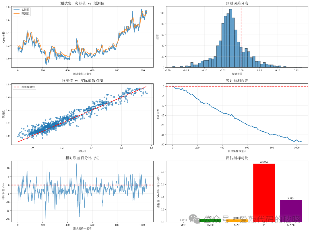
# 7. 评估指标对比柱状图
ax7 = plt.subplot(3, 3, 7)
metrics_to_plot = ['RMSE', 'MAE', 'MAPE', 'R2']
train_values = [train_metrics['RMSE'], train_metrics['MAE'],
train_metrics['MAPE'], train_metrics['R2']]
test_values = [test_metrics['RMSE'], test_metrics['MAE'],
test_metrics['MAPE'], test_metrics['R2']]
x = np.arange(len(metrics_to_plot))
width = 0.35
bars1 = ax7.bar(x - width/2, train_values, width, label='训练集', color='skyblue')
bars2 = ax7.bar(x + width/2, test_values, width, label='测试集', color='lightcoral')
ax7.set_title('评估指标对比', fontsize=14, fontweight='bold')
ax7.set_xticks(x)
ax7.set_xticklabels(metrics_to_plot)
ax7.set_ylabel('指标值 (MAPE为百分比)')
ax7.legend()
ax7.grid(True, alpha=0.3)
# 添加数值标签
for bars in [bars1, bars2]:
for bar in bars:
height = bar.get_height()
ax7.text(bar.get_x() + bar.get_width()/2., height,
f'{height:.2f}', ha='center', va='bottom', fontsize=9)
# 8. 预测误差时间序列
ax8 = plt.subplot(3, 3, 8)
ax8.plot(train_dates, train_errors, label='训练集误差', alpha=0.7)
ax8.axhline(y=0, color='r', linestyle='--', linewidth=1, alpha=0.5)
if len(train_dates) > 0 and len(test_dates) > 0:
ax8.axvline(x=separation_date, color='black', linestyle='--', linewidth=1, alpha=0.5)
ax8.set_title('预测误差时间序列', fontsize=14, fontweight='bold')
ax8.set_xlabel('日期')
ax8.set_ylabel('预测误差')
ax8.legend()
ax8.grid(True, alpha=0.3)
plt.setp(ax8.xaxis.get_majorticklabels(), rotation=45)
# 9. 残差Q-Q图(用于检验正态性)
ax9 = plt.subplot(3, 3, 9)
# 计算标准化残差
from scipy import stats
train_residuals = train_errors / np.std(train_errors)
test_residuals = test_errors / np.std(test_errors)
# 绘制Q-Q图
stats.probplot(train_residuals, dist="norm", plot=ax9)
ax9.get_lines()[0].set_markeredgecolor('blue')
ax9.get_lines()[0].set_alpha(0.6)
stats.probplot(test_residuals, dist="norm", plot=ax9)
ax9.get_lines()[2].set_marker('s')
ax9.get_lines()[2].set_markersize(4)
ax9.get_lines()[2].set_markerfacecolor('lightcoral')
ax9.get_lines()[2].set_markeredgecolor('red')
ax9.get_lines()[2].set_alpha(0.6)
# 自定义图例
legend_elements = [
Line2D([0], [0], marker='o', color='w', label='训练集残差',
markerfacecolor='skyblue', markersize=8),
Line2D([0], [0], color='black', linestyle='-', label='理论正态分布')
]
ax9.legend(handles=legend_elements)
ax9.set_title('残差Q-Q图(正态性检验)', fontsize=14, fontweight='bold')
ax9.grid(True, alpha=0.3)
plt.tight_layout()
plt.savefig('lstm_predictions_comprehensive.png', dpi=300, bbox_inches='tight')
plt.show()
# 单独显示密度散点图(大图)
fig_density, (ax_density1, ax_density2) = plt.subplots(1, 2, figsize=(16, 6))
plot_density_scatter(y_train_actual, train_predict, "训练集", ax_density1)
plot_density_scatter(y_test_actual, test_predict, "测试集", ax_density2)
plt.tight_layout()
plt.savefig('lstm_density_scatter_plots.png', dpi=300, bbox_inches='tight')
plt.show()
8.主函数模块
def main():
# 创建模型保存目录
if not os.path.exists('models'):
os.makedirs('models')
# 1. 读取CSV文件
filepath = 'AAC.AX.csv' # 请替换为您的文件路径
epochs = 10
try:
data_scaled, df, scaler = load_and_preprocess_data(filepath)
except FileNotFoundError:
print(f"错误:文件 '{filepath}' 未找到。请确保文件路径正确。")
return
except Exception as e:
print(f"读取文件时发生错误: {e}")
return
# 2. 创建时间序列数据集
look_back = 60 # 使用过去60天的数据预测下一天
X, y = create_dataset(data_scaled, look_back)
# 重塑数据以适应LSTM输入格式 [样本数, 时间步长, 特征数]
X = X.reshape(X.shape[0], X.shape[1], 1)
# 3. 划分训练集和测试集 (80:20)
train_size = int(len(X) * 0.8)
X_train, X_test = X[:train_size], X[train_size:]
y_train, y_test = y[:train_size], y[train_size:]
print(f"\n数据集划分:")
print(f"训练集形状: X_train={X_train.shape}, y_train={y_train.shape}")
print(f"测试集形状: X_test={X_test.shape}, y_test={y_test.shape}")
# 4. 检查是否有已训练的模型
model_path = 'models/lstm_model.h5'
scaler_path = 'models/scaler.pkl'
if os.path.exists(model_path) and os.path.exists(scaler_path):
print("\n发现已保存的模型,是否重新训练?")
choice = input("输入 'y' 重新训练,输入其他键使用现有模型: ").strip().lower()
if choice == 'y':
# 重新训练模型
print("\n开始重新训练模型...")
model = build_lstm_model((look_back, 1))
# 设置回调函数
callbacks = [
EarlyStopping(monitor='val_loss', patience=10, restore_best_weights=True),
ModelCheckpoint('models/best_lstm_model.h5', monitor='val_loss',
save_best_only=True, verbose=1)
]
# 训练模型
history = model.fit(
X_train, y_train,
epochs=epochs,
batch_size=32,
validation_split=0.1,
callbacks=callbacks,
verbose=1
)
# 保存模型
model.save(model_path)
joblib.dump(scaler, scaler_path)
print(f"模型已保存到 '{model_path}'")
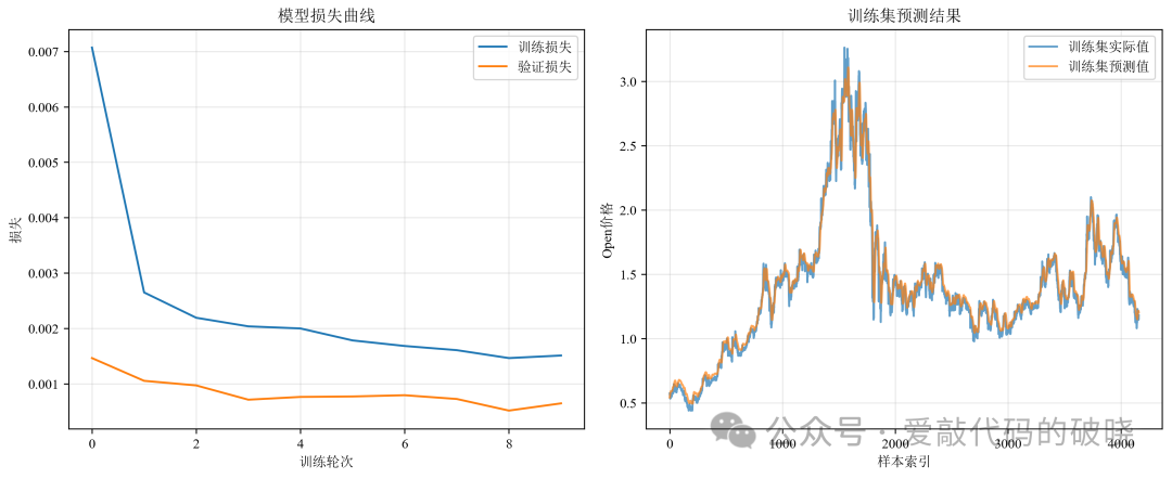
# 绘制训练历史
plt.figure(figsize=(10, 4))
plt.plot(history.history['loss'], label='训练损失')
plt.plot(history.history['val_loss'], label='验证损失')
plt.title('模型训练历史')
plt.xlabel('训练轮次')
plt.ylabel('损失')
plt.legend()
plt.grid(True, alpha=0.3)
plt.savefig('models/training_history.png', dpi=300, bbox_inches='tight')
plt.show()
else:
# 加载现有模型
else:
# 训练新模型
print("\n未找到已保存的模型,开始训练新模型...")
model = build_lstm_model((look_back, 1))
# 设置回调函数
callbacks = [
EarlyStopping(monitor='val_loss', patience=10, restore_best_weights=True),
ModelCheckpoint('models/best_lstm_model.h5', monitor='val_loss',
save_best_only=True, verbose=1)
]
# 训练模型
history = model.fit(
X_train, y_train,
epochs=epochs,
batch_size=32,
validation_split=0.1,
callbacks=callbacks,
verbose=1
)
# 保存模型
model.save(model_path)
joblib.dump(scaler, scaler_path)
print(f"模型已保存到 '{model_path}'")
# 5. 进行预测
print("\n进行预测...")
train_predict = model.predict(X_train)
test_predict = model.predict(X_test)
# 6. 反归一化
train_predict = scaler.inverse_transform(train_predict)
y_train_actual = scaler.inverse_transform(y_train.reshape(-1, 1))
test_predict = scaler.inverse_transform(test_predict)
y_test_actual = scaler.inverse_transform(y_test.reshape(-1, 1))
# 7. 评估预测结果
print("\n" + "="*50)
print("预测结果评估")
print("="*50)
train_metrics = evaluate_predictions(y_train_actual, train_predict, "训练集")
test_metrics = evaluate_predictions(y_test_actual, test_predict, "测试集")
# 8. 绘制所有图表
print("\n绘制图表...")
plot_predictions(df, train_predict, y_train_actual, test_predict,
y_test_actual, look_back, scaler, train_metrics, test_metrics)
# 9. 打印预测示例
print("\n" + "="*50)
print("预测结果示例")
print("="*50)
print(f"\n训练集前5个预测结果示例:")
print(f"{'索引':<8} {'实际值':<12} {'预测值':<12} {'误差':<12} {'相对误差(%)':<12}")
print("-" * 60)
for i in range(min(5, len(train_predict))):
actual = y_train_actual[i][0]
pred = train_predict[i][0]
error = actual - pred
rel_error = (error / actual) * 100
print(f"{i:<8} {actual:<12.4f} {pred:<12.4f} {error:<12.4f} {rel_error:<12.2f}")
print(f"\n测试集前5个预测结果示例:")
print(f"{'索引':<8} {'实际值':<12} {'预测值':<12} {'误差':<12} {'相对误差(%)':<12}")
print("-" * 60)
for i in range(min(5, len(test_predict))):
actual = y_test_actual[i][0]
pred = test_predict[i][0]
error = actual - pred
rel_error = (error / actual) * 100
print(f"{i:<8} {actual:<12.4f} {pred:<12.4f} {error:<12.4f} {rel_error:<12.2f}")
# 10. 保存预测结果到CSV文件
print("\n保存预测结果到CSV文件...")
9.运行结果展示
四、总结
LSTM的核心价值在于:
-
解决长期依赖问题:通过门控机制选择性记忆
-
捕捉复杂模式:非线性映射能力强
-
端到端学习:减少人工特征工程
-
灵活性高:可与其他模块结合(CNN、注意力等)


 1769
1769

 被折叠的 条评论
为什么被折叠?
被折叠的 条评论
为什么被折叠?
 到【灌水乐园】发言


