


今日任务:
- 网格搜索
- 随机搜索(简单介绍,非重点 实战中很少用到,可以不了解)
- 贝叶斯优化(2种实现逻辑,以及如何避开必须用交叉验证的问题)
- time库的计时模块,方便后人查看代码运行时长
-
对于信贷数据的其他模型,如LightGBM和KNN 尝试用贝叶斯优化和网格搜索调参
在完成了简单的建模和评估后,知道了模型的表现如何。但可能效果不理想(如过拟合或欠拟合),在更换模型前,可以考虑先调参。
一、数据读取与预处理
使用信贷数据集,读取数据:
import pandas as pd
#读取数据
data = pd.read_csv(r'data.csv')
data.info()
对数据进行简单预处理(数据类型转换、缺失值处理):
#数据预处理
#数据类型转换
discrete_features = data.select_dtypes(include=['object']).columns.tolist()
#标签编码
mapping_dict = {
    'Home Ownership':{
        'Own Home': 0,
        'Rent': 1,
        'Have Mortgage': 2,
        'Home Mortgage': 3
    },
    'Years in current job':{
        '< 1 year': 1,
        '1 year': 2,
        '2 years': 3,
        '3 years': 4,
        '4 years': 5,
        '5 years': 6,
        '6 years': 7,
        '7 years': 8,
        '8 years': 9,
        '9 years': 10,
        '10+ years': 11
    },
    'Term':{
        'Short Term':0,
        "Long Term":1
    }
}
for key,value in mapping_dict.items():
    data[key] = data[key].map(mapping_dict[key])

#独热编码
data = pd.get_dummies(data=data,columns=['Purpose'])
data2 = pd.read_csv("data.csv") # 重新读取数据,用来做列名对比
list_final = [] # 新建一个空列表,用于存放独热编码后新增的特征名
for i in data.columns:
    if i not in data2.columns:
       list_final.append(i) # 这里打印出来的就是独热编码后的特征名
for i in list_final:
    data[i] = data[i].astype(int) # 这里的i就是独热编码后的特征名

data.dtypes

#缺失值补全
continous_features = data.select_dtypes(include=['float64','int64']).columns.tolist()
for col in continous_features:
    mode_filled = data[col].mode()[0]
    data[col] = data[col].fillna(mode_filled)
data.isnull().sum()
二、数据集的划分
在调参的过程中,模型在间接地学习数据集的特征来调整超参数,如果只进行一次划分,那么最终得到的参数也只是碰巧在测试集表现很好,偶然性太大。故而在调参时,需要“考”2次,划分训练集、验证集和测试集。
- 训练集:用于训练模型。模型在这里学习数据中的内在规律和模式。
- 验证集:用于调参和模型选择。你在训练集上训练出多个不同参数或不同结构的模型,然后在验证集上评估它们,根据验证集的表现来选择最好的那一个。
- 测试集:用于最终评估。在你确定最终模型(包括结构和所有超参数)后,有且仅有一次地用测试集来评估它的性能,这个性能才被认为是模型泛化能力的真实反映。
#数据集的划分
from sklearn.model_selection import train_test_split
#标签与特征地确定
X = data.drop(['Credit Default'],axis=1)
y = data['Credit Default']

#划分两次数据集,得到训练集、验证集、训练集,比例为8:1:1
X_train,X_temp,y_train,y_temp = train_test_split(X,y,train_size=0.8,random_state=42)
X_val,X_test,y_val,y_test = train_test_split(X_temp,y_temp,train_size=0.5,random_state=42)但实际上,也可以选择使用‘交叉验证’的方法来提高模型的说服力,这个时候不需要划分验证集。常用的是K折交叉验证:将数据集均分为k份,每次取1份作为测试集,k-1份作为训练集,然后评估,共循环k次。最终取分数的平均值,作为模型的最终估计。
在很多调参方法中都默认有交叉验证(cross_val),实际中可只划分一次数据集:
#数据集的划分
from sklearn.model_selection import train_test_split
#标签与特征地确定
X = data.drop(['Credit Default'],axis=1)
y = data['Credit Default']
#划分一次数据集,得到测试集与训练集
X_train,X_test,y_train,y_test = train_test_split(X,y,train_size=0.7,random_state=42)
三、调参
调参能够为特定的数据集和任务,找到一组能使机器学习模型性能最佳、最稳定的超参数组合。
通过之前的学习,知道了模型与算法的区别,具体而言:模型 = 算法 + 实例化设置的外参 + 训练得到的内参。换言之,算法就像是一个通用的公式,而模型则是将具体数值代入公式后得到的结果。此外,在调参的过程中,要注意区分内参和外参,后者即超参数,是可以调整的参数:
- 参数:是模型内部根据数据自动学习得到的变量。例如,线性回归中的权重系数和偏置项,神经网络中的节点权重。我们不需要手动设置它们。
- 超参数:是模型外部的配置,在训练开始之前就必须由开发者手动设定。它们控制着模型的训练过程和行为。如学习率、树的最大深度等。
另外,在调参之前,需要确定一个基线模型,作为后续优化的比较基准:
- 未经任何优化、使用最常规设置(默认参数)的、能直接运行的模型。
- 设立一个科学、量化的“起点”,避免在后续工作中盲目优化,并展示出每一步工作的价值。
此处使用默认参数的RandomForestClassifier ():
#选择基线模型
from sklearn.ensemble import RandomForestClassifier
from sklearn.metrics import accuracy_score,precision_score,recall_score,f1_score
from sklearn.metrics import classification_report,confusion_matrix
import warnings #用于忽略警告信息
warnings.filterwarnings("ignore") # 忽略所有警告信息

import time #引入时间库,用于查看运行时间
print('默认随机森林训练结果:')
start_time = time.time()
rf_model = RandomForestClassifier(random_state=42) #实例化
rf_model.fit(X_train,y_train)
rf_pred = rf_model.predict(X_test)
end_time = time.time()
print('默认RF的训练时间:{:.2f}s'.format(end_time-start_time))
print('RF 分类报告:')
print(classification_report(y_true=y_test,y_pred=rf_pred))
print('RF 混淆矩阵:')
print(confusion_matrix(y_test,rf_pred))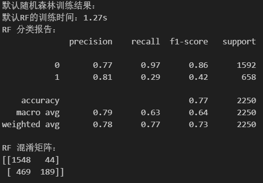
3.1 网格搜索(GridSearchCV)
指定一个超参数网格(param_grid),穷举所有可能的组合。效果可靠,但计算成本极高。因此,网格通常设置得比较小或集中在认为最优参数可能存在的区域(可能基于随机搜索的初步结果),适合在计算资源够用的情况。
使用网格搜索进行超参数调参的步骤:
- 定义参数网格param_grid:包含所有你想要尝试的特定值的列表,离散的;常见参数有n_estimators,max_depth,min_samples_split,min_samples_leaf
- 创建网格搜索对象:GridSearchCV();estimator,para_grid,cv,n_jobs,scoring参数含义看注释
- 训练集上进行网格搜索:grid_search.fit(X_train, y_train)
- 查看最佳参数(best_params_)、最佳模型(best_estimator_)
- 预测,查看评估指标
#网格搜索法调参
from sklearn.model_selection import GridSearchCV
start_time = time.time()
#定义参数网格
param_grid = {
'n_estimators': [50, 100, 200], #树的数量
'max_depth': [None, 10, 20, 30], #每棵树的最大深度
'min_samples_split': [2, 5, 10], #叶子结点所需的最小样本数
'min_samples_leaf': [1, 2, 4] #分裂内部节点所需地最小样本数
}
#创建网格搜索对象
grid_search = GridSearchCV(
estimator=RandomForestClassifier(random_state=42), #模型
param_grid=param_grid, #参数网格
cv=5, #K折交叉验证
n_jobs=-1, #可用的CPU核心,-1为全选
scoring='accuracy' #评分标准:准确率
)
#训练集上进行网格搜索
grid_search.fit(X_train,y_train)
end_time = time.time()
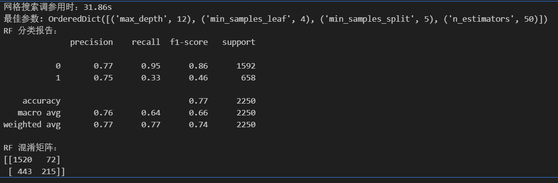
print('网格搜索调参用时:{:.2f}s'.format(end_time-start_time))
print("最佳参数:",grid_search.best_params_) #best_params_获取最佳参数
best_rf_model = grid_search.best_estimator_ #获得最佳模型
best_rf_pred = best_rf_model.predict(X_test) #测试集上进行预测
#评估
print('RF 分类报告:')
print(classification_report(y_true=y_test,y_pred=best_rf_pred))
print('RF 混淆矩阵:')
print(confusion_matrix(y_test,best_rf_pred))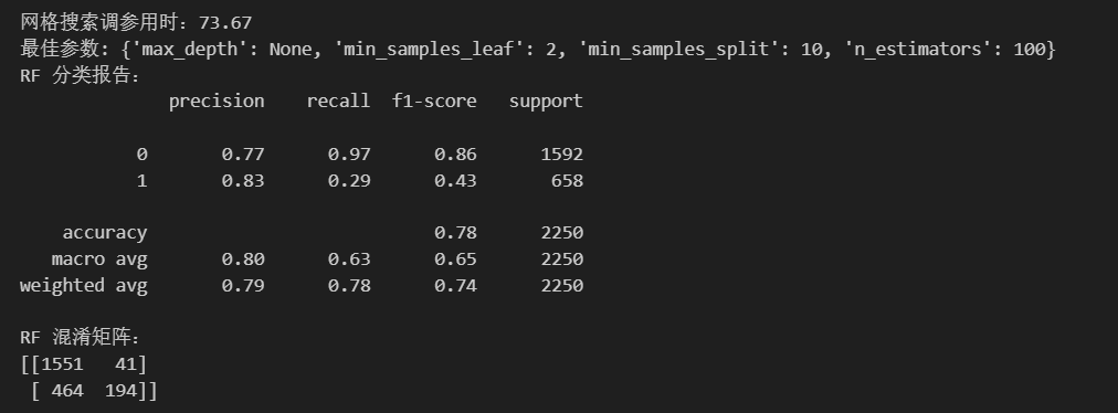
3.2 随机搜索(RandomizedSearchCV)
需要定义参数的分布,而不是固定的列表。在指定的参数空间中随机采样进行尝试,而不是尝试所有组合。对于给定的计算预算,随机搜索通常比网格搜索更有效,尤其是在高维参数空间中。
但是,随机搜索不常用。
3.3 贝叶斯优化(BayesSearchCV from skopt)
需要定义参数的搜索空间,根据之前的评估结果,建立概率模型来预测哪些超参数组合可能表现更好,并集中搜索这些区域。在寻找最优解方面通常比随机搜索更高效(用更少的迭代次数达到相似或更好的性能),特别是当模型训练(单次评估)非常耗时的时候,适合在计算资源不够用的情况
使用贝叶斯优化进行调参的步骤与网格搜索类似:
- 定义要搜索的参数空间search_space,参数空间是连续的
- 创建贝叶斯优化搜索对象BayesSearchCV(),参数与网格类似,多了一个迭代次数的调整
- 在训练集上进行贝叶斯优化搜索
- 最佳参数best_params_,最佳模型best_estimator_
-
预测,查看评估指标
#贝叶斯优化
from skopt import BayesSearchCV
from skopt.space import Integer
start_time = time.time()
#定义参数网格
search_space = {
'n_estimators': Integer(50,200),
'max_depth':Integer(10,30),
'min_samples_split': Integer(2,10),
'min_samples_leaf': Integer(1,4)
}
#创建网格搜索对象
bayes_search = BayesSearchCV(
estimator=RandomForestClassifier(random_state=42),#模型
search_spaces=search_space, #参数空间
n_iter=32, # 迭代次数,可根据需要调整
cv=5, #交叉验证
n_jobs=-1, #使用所有可用的CPU核心进行并行计算
scoring='accuracy'#使用准确率作为评分标准
)
#训练集上进行网格搜索
bayes_search.fit(X_train,y_train)
end_time = time.time()
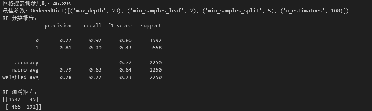
print('网格搜索调参用时:{:.2f}s'.format(end_time-start_time))
print("最佳参数:",bayes_search.best_params_)#best_params_属性返回最佳参数组合
best_rf_model = bayes_search.best_estimator_ #获取最佳模型
best_rf_pred = best_rf_model.predict(X_test) #在测试集上进行预测
#评估
print('RF 分类报告:')
print(classification_report(y_true=y_test,y_pred=best_rf_pred))
print('RF 混淆矩阵:')
print(confusion_matrix(y_test,best_rf_pred))此处应该为贝叶斯优化:
3.4 贝叶斯优化的其它实现方法(了解)
下面介绍一种贝叶斯优化方法的其他实现代码,他的优势在于:
- 可以自己定义目标函数,也可以借助他不使用交叉验证,因为评估指标修改为不是交叉验证的结果即可,更加自由
- 有verbose参数,可以输出中间过程
# --- 2. 贝叶斯优化随机森林 ---
print("\n--- 2. 贝叶斯优化随机森林 (训练集 -> 测试集) ---")
from bayes_opt import BayesianOptimization
from sklearn.ensemble import RandomForestClassifier
from sklearn.model_selection import cross_val_score
from sklearn.metrics import classification_report, confusion_matrix
import time
import numpy as np
# 假设 X_train, y_train, X_test, y_test 已经定义好
# 定义目标函数,这里使用交叉验证来评估模型性能
def rf_eval(n_estimators, max_depth, min_samples_split, min_samples_leaf):
n_estimators = int(n_estimators)
max_depth = int(max_depth)
min_samples_split = int(min_samples_split)
min_samples_leaf = int(min_samples_leaf)
model = RandomForestClassifier(
n_estimators=n_estimators,
max_depth=max_depth,
min_samples_split=min_samples_split,
min_samples_leaf=min_samples_leaf,
random_state=42
)
scores = cross_val_score(model, X_train, y_train, cv=5, scoring='accuracy')
return np.mean(scores)
# 定义要搜索的参数空间
pbounds_rf = {
'n_estimators': (50, 200),
'max_depth': (10, 30),
'min_samples_split': (2, 10),
'min_samples_leaf': (1, 4)
}
# 创建贝叶斯优化对象,设置 verbose=2 显示详细迭代信息
optimizer_rf = BayesianOptimization(
f=rf_eval, # 目标函数
pbounds=pbounds_rf, # 参数空间
random_state=42, # 随机种子
verbose=2 # 显示详细迭代信息
)
start_time = time.time()
# 开始贝叶斯优化
optimizer_rf.maximize(
init_points=5, # 初始随机采样点数
n_iter=32 # 迭代次数
)
end_time = time.time()
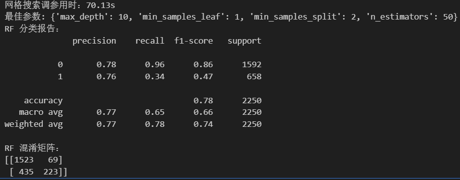
print(f"贝叶斯优化耗时: {end_time - start_time:.4f} 秒")
print("最佳参数: ", optimizer_rf.max['params'])
# 使用最佳参数的模型进行预测
best_params = optimizer_rf.max['params']
best_model = RandomForestClassifier(
n_estimators=int(best_params['n_estimators']),
max_depth=int(best_params['max_depth']),
min_samples_split=int(best_params['min_samples_split']),
min_samples_leaf=int(best_params['min_samples_leaf']),
random_state=42
)
best_model.fit(X_train, y_train)
best_pred = best_model.predict(X_test)
print("\n贝叶斯优化后的随机森林 在测试集上的分类报告:")
print(classification_report(y_test, best_pred))
print("贝叶斯优化后的随机森林 在测试集上的混淆矩阵:")
print(confusion_matrix(y_test, best_pred))四、作业:对LightGBM模型进行调参
使用网格搜索和贝叶斯优化对LightGBM模型进行调参。
网格搜索
#LGBM网格搜索法调参
from lightgbm import LGBMClassifier
from sklearn.model_selection import GridSearchCV
start_time = time.time()
#定义参数网格
param_grid = {
    'n_estimators': [50, 100, 200],
    'max_depth': [None, 10, 20, 30],
    'min_samples_split': [2, 5, 10],
    'min_samples_leaf': [1, 2, 4]
}
#创建网格搜索对象
grid_search = GridSearchCV(
    estimator=LGBMClassifier(random_state=42),
    param_grid=param_grid,
    cv=5,
    n_jobs=-1,
    scoring='accuracy'
)
#训练集上进行网格搜索
grid_search.fit(X_train,y_train)

end_time = time.time()
print('网格搜索调参用时:{:.2f}s'.format(end_time-start_time))

print("最佳参数:",grid_search.best_params_)

best_rf_model = grid_search.best_estimator_
best_rf_pred = best_rf_model.predict(X_test)

#评估
print('RF 分类报告:')
print(classification_report(y_true=y_test,y_pred=best_rf_pred))
print('RF 混淆矩阵:')
print(confusion_matrix(y_test,best_rf_pred))
此处应为LGBM:
贝叶斯优化
#LGBM贝叶斯优化
from skopt import BayesSearchCV
from skopt.space import Integer

start_time = time.time()
#定义参数网格
search_space = {
    'n_estimators': Integer(50,200),
    'max_depth':Integer(10,30),
    'min_samples_split': Integer(2,10),
    'min_samples_leaf': Integer(1,4)
}
#创建网格搜索对象
bayes_search = BayesSearchCV(
    estimator=LGBMClassifier(random_state=42),
    search_spaces=search_space,
    n_iter=32,  # 迭代次数,可根据需要调整
    cv=5,
    n_jobs=-1,
    scoring='accuracy'
)
#训练集上进行网格搜索
bayes_search.fit(X_train,y_train)

end_time = time.time()
print('网格搜索调参用时:{:.2f}s'.format(end_time-start_time))

print("最佳参数:",bayes_search.best_params_)

best_rf_model = bayes_search.best_estimator_
best_rf_pred = best_rf_model.predict(X_test)

#评估
print('RF 分类报告:')
print(classification_report(y_true=y_test,y_pred=best_rf_pred))
print('RF 混淆矩阵:')
print(confusion_matrix(y_test,best_rf_pred))
此处应该为贝叶斯优化与LGBM:
根据对LGBM采用网格搜索和贝叶斯优化进行调参对比后发现,虽然两者整体思路类似,但是贝叶斯优化方法比网格搜索快了一倍,更加高效。


 1万+
1万+

 被折叠的 条评论
为什么被折叠?
被折叠的 条评论
为什么被折叠?
 到【灌水乐园】发言


