


今日任务:
- 方差筛选
- 皮尔逊相关系数筛选
- lasso筛选
- 树模型重要性
- shap重要性
- 递归特征消除REF
作业:对心脏病数据集完成特征筛选,对比精度
对于许多数据来说,它们拥有众多的特征,如果不进行处理,就会出现计算速度下降以及冗余特征的干扰等问题。因此,对于高维特征的数据,特征降维十分必要。
常见的特征降维方法主要有两种:
- 特征筛选:从n个特征中筛选出m个特,包括过滤法、包裹法及嵌入法等
- 特征组合:从n个特征组合出m个特征,如PCA
今日主要学习特征筛选,它适合于不相关特征、冗余特征和噪声特征的处理。下面是三类常用的特征筛选方法的介绍:
- 过滤法:基于特征的统计属性(如方差、相关性、互信息)进行筛选。如方差选择法、相关系数法、卡方检验、互信息法。
- 包裹法:将模型本身的性能作为评价标准,通过不断尝试不同的特征子集,选择使模型性能最佳的特征组合。如递归特征消除(RFE)、前向选择、后向剔除。
- 嵌入法:将特征选择过程与模型训练过程融为一体。模型在训练时会自动进行特征选择。如使用L1正则化(Lasso回归)的模型、决策树/随机森林/Gradient Boosting模型提供的特征重要性。
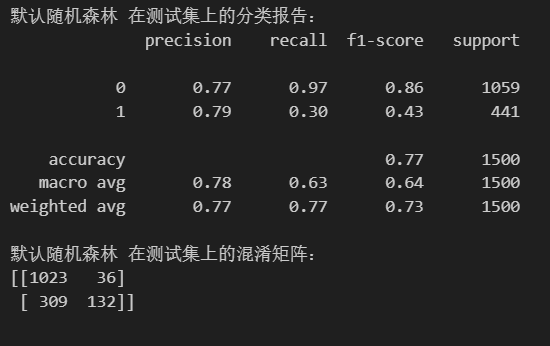
首先对信贷数据集使用默认参数的随机森林训练得到下面的结果:
下面是具体的六种方法的说明,以及特征筛选后的结果:
方差筛选
过滤式无监督,通过计算数据的方差大小和阈值(认为设定)进行比较,大于则保留,小于则删去。它的核心思想基于下面的假设:如果一个特征在不同的样本中的取值几乎没有变化(方差值很小),那么它能提供的区分样本的信息量就很少,故而该特征对模型的预测能力的贡献就几乎忽略不计。
方差筛选法可以通过sklearn库中VarienceThreshold(threshold=0.0)完成。
#方差筛选法
from sklearn.feature_selection import VarianceThreshold
start_time = time.time()
selector = VarianceThreshold(threshold=0.01) #实例化
X_train_var = selector.fit_transform(X_train) #训练并转换原始训练集
X_test_var = selector.transform(X_test) #转换测试集
#查看筛选后的特征
selected_features_var = X_train.columns[selector.get_support()].tolist() #X_train.columns[selector.get_support()]的类型
#print('筛选的特征:{},长度:{}'.format(selected_features_var,len(selected_features_var)))
#重新训练模型
rf_model_var = RandomForestClassifier(random_state=42)
rf_model_var.fit(X_train_var,y_train)
rf_pred_var = rf_model_var.predict(X_test_var)
end_time = time.time()
print(f"训练与预测耗时: {end_time - start_time:.4f} 秒")
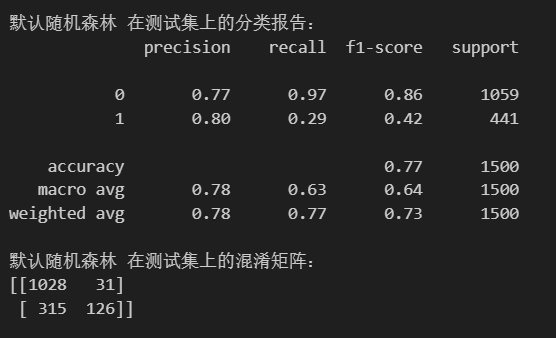
print("\n默认随机森林 在测试集上的分类报告:")
print(classification_report(y_test, rf_pred_var))
print("默认随机森林 在测试集上的混淆矩阵:")
print(confusion_matrix(y_test, rf_pred_var))
特征筛选后,得到21个特征,训练结果与之前差异不大:
根据定义,可以看出方差筛选法的优缺点:
- 优点:计算速度较快;简单易懂;不需要标签,在预处理阶段可完成
- 缺点:阈值选择困难;忽略特征与目标的关系,只关注特征本身的分布;对特征尺度敏感
皮尔逊相关系数筛选
过滤式有监督,通过量化每个特征与目标变量之间的线性关系强度,来筛选出与目标最相关的特征,同时也可以用于提出高度相关的冗余特征。需要注意的是它处理的目标变量为连续性,若为离散型需要进行编码处理,转换为数据型。
判断线性关系程度与方向的指标是皮尔逊相关系数(r),取值范围是[-1,1]:
- 方向:r = 1表示完全正相关,一个变量增加,另一个变量也线性增加。r = -1表示完全负相关,一个变量增加,另一个变量线性减少。 r =0表示没有线性相关关系。
- 强度:|r| ≥ 0.8,强相关;0.5 ≤ |r| < 0.8,中等相关;0.3 ≤ |r| < 0.5,弱相关;|r| < 0.3,极弱相关或无相关。
这里使用SelectKBest(score_func=f_classif,k=k)来筛选前k个特征。其中f_classif为评分函数,计算的是每个特征与目标变量之间的ANOVA F值(方差分析F值),用于衡量特征在不同类别间的差异程度。
#皮尔逊系数筛选
from sklearn.feature_selection import SelectKBest,f_classif
start_time = time.time()
k = 10
selector = SelectKBest(score_func=f_classif,k=k) #实例化
X_train_corr = selector.fit_transform(X_train,y_train) #训练并转换训练集
X_test_corr = selector.transform(X_test) #转换测试集
#查看筛选的特征
selected_features_corr = X_train.columns[selector.get_support()].tolist()
print('筛选的特征:{},\n长度:{}'.format(selected_features_corr,len(selected_features_corr)))
rf_model_corr = RandomForestClassifier(random_state=42)
rf_model_corr.fit(X_train_corr,y_train)
rf_pred_corr = rf_model_corr.predict(X_test_corr)
end_time = time.time()
print(f"训练与预测耗时: {end_time - start_time:.4f} 秒")
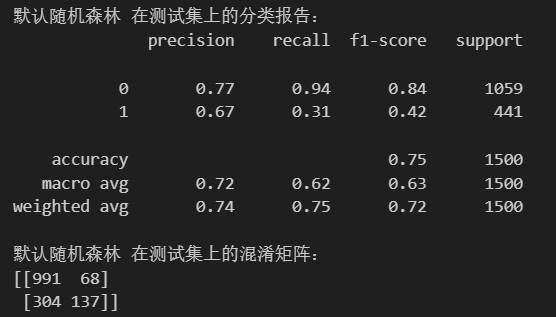
print("\n默认随机森林 在测试集上的分类报告:")
print(classification_report(y_test, rf_pred_corr))
print("默认随机森林 在测试集上的混淆矩阵:")
print(confusion_matrix(y_test, rf_pred_corr))皮尔逊系数筛选后剩余10个特征,在训练效果上有所差异:
lasso筛选(基于L1正则化)
Lasso(Least Absolute Shrinkage and Selection Operator,即最小绝对收缩和选择算子)筛选,它的核心思想是在线性回归的同时,通过引入L1正则化项(惩罚项),强制将一些不重要特征的回归系数压缩到0,从而实现特征筛选。
也就是说,Lasso会自动“挑选”对预测目标有贡献的特征(系数不为0),而剔除无关或冗余的特征(系数为0)。
lasso筛选的实现可以通过SelectFromModel包装器,基于LASSO模型的系数来自动选择重要特征:
- SelectFromModel:元转换器,自动设置阈值(默认为中位数),只保留那些重要性高于改阈值的特征。相比直接使用LASSO系数(手动),可以自动选择重要特征
- Lasso:创建LASSO回归模型,alpha为正则化强度参数,alpha越大,正则化越强,保留的特征越少
#lasso筛选
from sklearn.linear_model import Lasso
from sklearn.feature_selection import SelectFromModel
start_time = time.time()
#创建Lasso模型
lasso = Lasso(alpha=0.01,random_state=42) #alpha正则化强度参数
selector = SelectFromModel(estimator=lasso) #包装器
selector.fit(X_train,y_train) #训练
X_train_lasso = selector.transform(X_train) #转换训练集
X_test_lasso = selector.transform(X_test) #转换测试集
#查看特征
selected_features_lasso = X_train.columns[selector.get_support()].tolist()
print('筛选的特征:{},\n长度:{}'.format(selected_features_lasso,len(selected_features_lasso)))
#重新训练模型
rf_model_lasso = RandomForestClassifier(random_state=42)
rf_model_lasso.fit(X_train_lasso,y_train)
rf_pred_lasso = rf_model_lasso.predict(X_test_lasso)
end_time = time.time()
print(f"训练与预测耗时: {end_time - start_time:.4f} 秒")
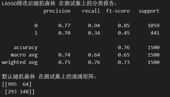
print("\nLASSO筛选后随机森林 在测试集上的分类报告:")
print(classification_report(y_test, rf_pred_lasso))
print("默认随机森林 在测试集上的混淆矩阵:")
print(confusion_matrix(y_test, rf_pred_lasso))
经过lasso筛选后,得到7个特征:
树模型的重要性
属于嵌入性,这个是树模型自带的重要性筛选。
同样地,借助SelectFromModel(estimator,threshold,...)包装器,完成特征筛选工作。一般步骤是:(1)建立模型(2)包装器筛选(3)训练、转换(4)查看筛选后的特征名,借助selector.get_support()布尔掩码(5)使用筛选后的特征训练,对比前后结果
#树模型筛选重要性
from sklearn.ensemble import RandomForestClassifier
from sklearn.feature_selection import SelectFromModel

start_time = time.time()
#创建rf模型
rf_selector = RandomForestClassifier(random_state=42)
rf_selector.fit(X_train,y_train)
selector = SelectFromModel(estimator=rf_selector)
X_train_rf = selector.transform(X_train) #转换训练集
X_test_rf = selector.transform(X_test) #转换测试集
#查看特征
selected_features_rf = X_train.columns[selector.get_support()].tolist()
print('筛选的特征:{},\n长度:{}'.format(selected_features_rf,len(selected_features_rf)))
#重新训练模型
rf_model_rf = RandomForestClassifier(random_state=42)
rf_model_rf.fit(X_train_rf,y_train)
rf_pred_rf = rf_model_rf.predict(X_test_rf)
end_time = time.time()

print(f"训练与预测耗时: {end_time - start_time:.4f} 秒")
print("\n树模型自带筛选后随机森林 在测试集上的分类报告:")
print(classification_report(y_test, rf_pred_rf))
print("默认随机森林 在测试集上的混淆矩阵:")
print(confusion_matrix(y_test, rf_pred_rf))
通过筛选后,剩余11个特征:

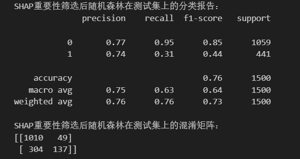
SHAP重要性筛选
基于SHAP值的模型解释性的高级特征选择方法。根据每个特征对模型预测的贡献度大小,选择最重要的k个特征。
具体步骤如下:(1)训练模型并创建shap解释器(2)计算shap值(3)计算特征重要性并选择top-k特征(4)使用特征索引选择训练集和测试集的对应特征iloc (5)重新训练,对比结果
通过SHAP筛选后,剩余10个特征:
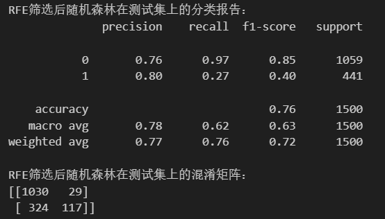
递归特征消除RFE
递归特征消除法(Recursive Feature Elimination,RFE),属于包裹法,通过递归地构建模型并剔除最不重要的特征,最终保留最优的特征子集。它是一个反复迭代的过程,每次迭代都会训练一个模型,根据特征重要性排序,淘汰掉最不重要的特征,直到达到指定的特征数量。
通过RFE筛选后,剩余10个特征:
下面是六种方法的总结:
| 方法 | 类型 | 监督性 | 计算成本 | 核心原理 | 是否考虑特征交互 |
|---|---|---|---|---|---|
| 方差筛选 | 过滤法 | 无监督 | 很低 | 特征本身的方差大小 | 否 |
| 皮尔逊系数筛选 | 过滤法 | 有监督 | 低 | 特征与目标的线性相关性 | 否 |
| LASSO筛选 | 嵌入法 | 有监督 | 中 | L1正则化压缩系数为0 | 是(线性) |
| 树模型筛选 | 嵌入法 | 有监督 | 中 | 基于分裂增益的重要性 | 是 |
| SHAP筛选 | 模型解释 | 有监督 | 高 | 基于博弈论的边际贡献 | 是 |
| 递归特征消除(RFE) | 包裹法 | 有监督 | 很高 | 递归剔除最不重要特征 | 是 |
作业:心脏病特征筛选
总结一下,使用上述六种方法进行特征筛选时,基本的步骤相似:
- 导入所需要的库
- 创建模型,确定是否需要包装器等辅助
- 训练、转换训练集与测试集
- 借助selector.get_support()查看筛选特征后的结果
- 重新训练模型,比对结果
今日时间有限,明日续上今日剩余部分


 933
933

 被折叠的 条评论
为什么被折叠?
被折叠的 条评论
为什么被折叠?
 到【灌水乐园】发言


