Day 34 GPU训练及类的call方法

最新推荐文章于 2025-11-24 15:28:47 发布

原创最新推荐文章于 2025-11-24 15:28:47 发布 · 1k 阅读

25 ·

CC 4.0 BY-SA版权

文章标签：

#python #神经网络 #深度学习

Python打卡训练营专栏收录该内容

52 篇文章

订阅专栏

@浙大疏锦行

今日任务：

CPU性能的查看：看架构代际、核心数、线程数
GPU性能的查看：看显存、看级别、看架构代际
GPU训练的方法：数据和模型移动到GPU device上
类的call方法：为什么定义前向传播时可以直接写作self.fc1(x)

ps：在训练过程中可以在命令行输入nvida-smi查看显存占用情况

先简单回顾昨天学习的简单神经网络流程：

（1）准备数据（2）数据预处理：归一化、张量转换（3）模型框架定义：继承类；定义输出层/隐藏层/输入层；前向传播（3）损失函数和优化器的创建（4）循环训练：确定训练轮数；循环内部过程（forward,loss,backward,step）（5）可视化损失函数，查看收敛情况

CPU和GPU性能查看

【深度学习小常识】CPU（中央处理器）和GPU（图像处理器）的区别

CPU

import wmi
c = wmi.WMI()
processors = c.Win32_Processor()
for processor in processors:
    print(f"CPU 型号: {processor.Name}") 
    print(f"核心数: {processor.NumberOfCores}")
    print(f"线程数: {processor.NumberOfLogicalProcessors}")

GPU

GPU训练

GPU的并行计算能力强，训练神经网络可以提速10-100倍。要想让模型在GPU上训练，需要将模型和数据(张量)迁移到GPU设备上，使用的方法是.to(device)。
考虑到代码的可移植性和鲁棒性（不是所有人都有GPU），使用如下写法，确定device设备：

device = torch.device("cuda:0" if torch.cuda.is_available() else "cpu")
print(f"使用设备: {device}")

模型/数据迁移

确定好设备后，就需要将数据和模型迁移至设备上。需要注意的是，所有需要在GPU/CPU上做计算的核心对象都支持.to(device)，如Tensor（张量）及子类、nn.Module及子类（模型，并且要保证这些对象迁移到同一个设备上。

#张量转换，迁移至GPU
X_train = torch.FloatTensor(X_train).to(device)
X_test = torch.FloatTensor(X_test).to(device)
y_train = torch.LongTensor(y_train).to(device)
y_test = torch.LongTensor(y_test).to(device)

#实例化，迁移至设备
model = MLP().to(device)

完整版

# GPU版本
from sklearn.datasets import load_iris
from sklearn.model_selection import train_test_split
from sklearn.preprocessing import MinMaxScaler
import torch
import torch.nn as nn
import torch.optim as optim

# 设置设备
device = torch.device('cuda:0' if torch.cuda.is_available() else 'cpu')
print(f'使用的设备：{device}')

# 数据准备
iris = load_iris() 
X = iris.data # 特征
y = iris.target # 标签
X_train,X_test,y_train,y_test = train_test_split(X,y,test_size=0.2,random_state=42) # 划分数据集

# 数据预处理
#归一化
scaler = MinMaxScaler()
X_train = scaler.fit_transform(X_train)
X_test = scaler.transform(X_test)
#张量转换，迁移至GPU
X_train = torch.FloatTensor(X_train).to(device)
X_test = torch.FloatTensor(X_test).to(device)
y_train = torch.LongTensor(y_train).to(device)
y_test = torch.LongTensor(y_test).to(device)

# 模型框架定义
class MLP(nn.Module): # 继承nn.Module类
    def __init__(self): # 初始化
        super(MLP,self).__init__() #调用父类方法
        #定义每一层
        self.fc1 = nn.Linear(4,10)
        self.relu = nn.ReLU()
        self.fc2 = nn.Linear(10,3)
    #定义前向传播
    def forward(self,x):
        out = self.fc1(x)
        out = self.relu(out)
        out = self.fc2(out)
        return out
#实例化，迁移至设备
model = MLP().to(device)

# 损失函数和优化器
criterion = nn.CrossEntropyLoss() # 损失函数
optimiser = optim.SGD(model.parameters(), lr=0.01) # SGD
#optimiser = optim.Adam(model.parameters(),lr=0.001) # Adam

# 循环训练
epoch_num = 20000 # 训练轮数
losses = []
import time
start_time = time.time()
for epoch in range(epoch_num):
    output = model(X_train) # 隐式调用forward方法
    loss = criterion(output,y_train)
    #反向传播
    optimiser.zero_grad() # 清零
    loss.backward() # 反向传播计算梯度
    optimiser.step() # 更新参数
    # 记录loss值
    losses.append(loss.item())

    # 打印
    if (epoch + 1) % 100 == 0: # range是从0开始，所以epoch+1是从当前epoch开始，每100个epoch打印一次
        print(f'Epoch [{epoch+1}/{epoch_num}], Loss: {loss.item():.4f}')

time_all = time.time() - start_time # 计算训练时间
print(f'The training time of CPU: {time_all:.2f} seconds')
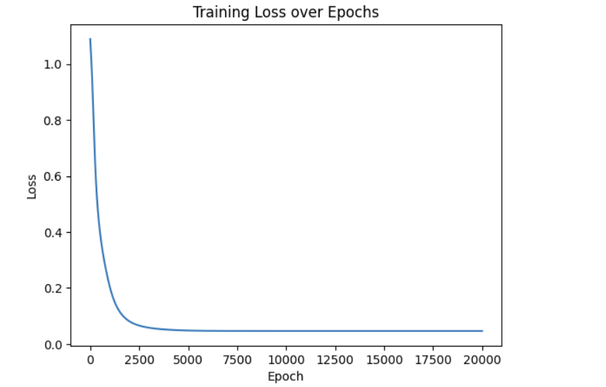
# 可视化
import matplotlib.pyplot as plt
plt.plot(list(range(epoch_num)),losses)
plt.xlabel('Epoch')
plt.ylabel('Loss')
plt.title('Training Loss over Epochs')
plt.show()

Adam优化器：

计算开销

租用云服务器RTX-4090，CPU版本用时4.15s，GPU版本用时9.59s。

对于极小的数据集（如鸢尾花数据），CPU的运行速度快于GPU，主要是因为GPU运行时存在固定的计算开销：

数据传输开销：CPU 内存 ↔ GPU 显存之间的数据拷贝。GPU计算前，数据从RAM到VRAM；结果返回时，从GPU到CPU，比如loss.item()（把标量从GPU到CPU,触发同步）
核心启动开销：GPU 执行的每个操作（Linear + ReLU + Linear）都涉及到在 GPU 上启动一个“核心”(kernel)——一个在 GPU 众多计算单元上运行的小程序，存在固定开销。
性能浪费：数据量太少时，GPU的很多计算单元都没有被用到，即使用了全批次也没有用到的全部计算单元。

综上，对于小数据集来说，GPU固定的计算开销远大于它在速度上的提升，因此在这个情况下速度反而慢于CPU。

GPU能发挥优势的场景主要集中在大批量数据处理，能发挥并行性优势：

大型数据集：例如，图像数据集成千上万张图片，每张图片维度很高。
大型模型：例如，深度卷积网络 (CNNs like ResNet, VGG) 或 Transformer 模型，它们有数百万甚至数十亿的参数，计算量巨大。
合适的批处理大小：能够充分利用 GPU 并行性的 batch size，不至于还有剩余的计算量没有被 GPU 处理。
复杂的、可并行的运算：大量的矩阵乘法、卷积等。

优化

对于固定的流程和数据，能够优化的只有数据传输这一步了，考虑到loss.item()每次循环都会进行从GPU到CPU的过程，可能累积大量时间，从这个优化入手：

（1）直接去除，但是无法可视化，用时8.62s。

# GPU-修改版
from sklearn.datasets import load_iris
from sklearn.model_selection import train_test_split
from sklearn.preprocessing import MinMaxScaler
import torch
import torch.nn as nn
import torch.optim as optim

# 设置设备
device = torch.device('cuda:0' if torch.cuda.is_available() else 'cpu')
print(f'使用的设备：{device}')

# 数据准备
iris = load_iris() 
X = iris.data # 特征
y = iris.target # 标签
X_train,X_test,y_train,y_test = train_test_split(X,y,test_size=0.2,random_state=42) # 划分数据集

# 数据预处理
#归一化
scaler = MinMaxScaler()
X_train = scaler.fit_transform(X_train)
X_test = scaler.transform(X_test)
#张量转换，迁移至GPU
X_train = torch.FloatTensor(X_train).to(device)
X_test = torch.FloatTensor(X_test).to(device)
y_train = torch.LongTensor(y_train).to(device)
y_test = torch.LongTensor(y_test).to(device)

# 模型框架定义
class MLP(nn.Module): # 继承nn.Module类
    def __init__(self): # 初始化
        super(MLP,self).__init__() #调用父类方法
        #定义每一层
        self.fc1 = nn.Linear(4,10)
        self.relu = nn.ReLU()
        self.fc2 = nn.Linear(10,3)
    #定义前向传播
    def forward(self,x):
        out = self.fc1(x)
        out = self.relu(out)
        out = self.fc2(out)
        return out
#实例化，迁移至设备
model = MLP().to(device)

# 损失函数和优化器
criterion = nn.CrossEntropyLoss() # 损失函数
optimiser = optim.SGD(model.parameters(), lr=0.01) # SGD
#optimiser = optim.Adam(model.parameters(),lr=0.001) # Adam

# 循环训练
epoch_num = 20000 # 训练轮数
losses = []
import time
start_time = time.time()
for epoch in range(epoch_num):
    output = model(X_train) # 隐式调用forward方法
    loss = criterion(output,y_train)
    #反向传播
    optimiser.zero_grad() # 清零
    loss.backward() # 反向传播计算梯度
    optimiser.step() # 更新参数
    # 记录loss值
    #losses.append(loss.item())

    # 打印
    if (epoch + 1) % 100 == 0: # range是从0开始，所以epoch+1是从当前epoch开始，每100个epoch打印一次
        print(f'Epoch [{epoch+1}/{epoch_num}], Loss: {loss.item():.4f}')

time_all = time.time() - start_time # 计算训练时间
print(f'The training time of CPU: {time_all:.2f} seconds')
# 可视化

（2）减少次数访问（保留可视化），每隔N步记录一次（间隔200）

# GPU-修改版
from sklearn.datasets import load_iris
from sklearn.model_selection import train_test_split
from sklearn.preprocessing import MinMaxScaler
import torch
import torch.nn as nn
import torch.optim as optim

# 设置设备
device = torch.device('cuda:0' if torch.cuda.is_available() else 'cpu')
print(f'使用的设备：{device}')

# 数据准备
iris = load_iris() 
X = iris.data # 特征
y = iris.target # 标签
X_train,X_test,y_train,y_test = train_test_split(X,y,test_size=0.2,random_state=42) # 划分数据集

# 数据预处理
#归一化
scaler = MinMaxScaler()
X_train = scaler.fit_transform(X_train)
X_test = scaler.transform(X_test)
#张量转换，迁移至GPU
X_train = torch.FloatTensor(X_train).to(device)
X_test = torch.FloatTensor(X_test).to(device)
y_train = torch.LongTensor(y_train).to(device)
y_test = torch.LongTensor(y_test).to(device)

# 模型框架定义
class MLP(nn.Module): # 继承nn.Module类
    def __init__(self): # 初始化
        super(MLP,self).__init__() #调用父类方法
        #定义每一层
        self.fc1 = nn.Linear(4,10)
        self.relu = nn.ReLU()
        self.fc2 = nn.Linear(10,3)
    #定义前向传播
    def forward(self,x):
        out = self.fc1(x)
        out = self.relu(out)
        out = self.fc2(out)
        return out
#实例化，迁移至设备
model = MLP().to(device)

# 损失函数和优化器
criterion = nn.CrossEntropyLoss() # 损失函数
optimiser = optim.SGD(model.parameters(), lr=0.01) # SGD
#optimiser = optim.Adam(model.parameters(),lr=0.001) # Adam

# 循环训练
epoch_num = 20000 # 训练轮数
losses = []
import time
start_time = time.time()
for epoch in range(epoch_num):
    output = model(X_train) # 隐式调用forward方法
    loss = criterion(output,y_train)
    #反向传播
    optimiser.zero_grad() # 清零
    loss.backward() # 反向传播计算梯度
    optimiser.step() # 更新参数
        
    # 打印
    if (epoch + 1) % 100 == 0: # range是从0开始，所以epoch+1是从当前epoch开始，每100个epoch打印一次
        print(f'Epoch [{epoch+1}/{epoch_num}], Loss: {loss.item():.4f}')
    # 记录loss值
    if (epoch + 1) % 200 == 0:
        losses.append(loss.item()) # item()方法返回一个Python数值，loss是一个标量张量

time_all = time.time() - start_time # 计算训练时间
print(f'The training time of CPU: {time_all:.2f} seconds')
# 可视化
import matplotlib.pyplot as plt
plt.plot(range(len(losses)), losses)
plt.xlabel('Epoch')
plt.ylabel('Loss')
plt.title('Training Loss over Epochs')
plt.show()

（3）记录间隔和时长的关系

版本	时间（SGD）	时间（Adam）
CPU	4.53 s	7.49 s
GPU	9.37 s	12.27 s
GPU-1	8.81 s	12.59 s
GPU-2	9.29 s	11.01 s

记录间隔（轮）	200	400	500	800	1000	1250	2000
记录次数（次）	100	50	40	25	20	16	10
时间	9.29 s	9.00 s	8.96 s	8.97 s	9.10 s	9.13 s	8.69 s

总体上，呈现的是记录间隔越大，时间越短的规律。根本原因是loss.item() 触发 GPU-CPU 同步（gpu需要等待cpu完成才能开启下次运算），记录间隔越小 → loss.item() 越频繁 → 同步越多 → GPU 利用率下降 → 总时间增加。

但是存在波动，存在其它因素影响（AI分析）：

因素	说明	是否导致波动
`.item()` 同步开销	每次调用阻塞 GPU，耗时约 1~10 μs	主导趋势
GPU 调度随机性	CUDA kernel 启动顺序、资源竞争等	导致微小波动
显存访问模式	不同 batch 或 epoch 下缓存命中率不同	影响性能
PyTorch 缓存分配器行为	首次分配 vs 再利用显存	可能引入差异
系统负载变化	其他进程占用 GPU/CPU/内存	外部干扰

魔术方法call

在定义模型的基本框架时，可以注意到，self.fc1 = nn.Linear(4, 10) 此时，是实例化了一个nn.Linear(4, 10)对象，并把这个对象赋值给了MLP的初始化函数中的self.fc1变量。然后， out = self.fc1(x)，这个self.fc1这个变量却实现了函数的用法？

这是因为nn.Linear继承了nn.Module类，nn.Module类中定义了__call__方法。PyTorch 中几乎所有层（nn.Linear, nn.ReLU, nn.Conv2d 等）都是 nn.Module 的子类，所以它们的实例也都有__call__方法，可以像函数一样调用。

__call__方法：让实例对象像函数一样被调用。不管有没有参数，只要有call方法，那么实例对象就可以像函数一样被使用。

class Adder:
    def __init__(self):
        self.count = 0
    #def __call__(self): # 无参数的call方法，在每次调用实例后自动触发
        #self.count += 1
        return self.count
    def __call__(self, a, b): # 有参数的call方法
        return a + b

add = Adder() # 创建实例对象
result = add(3, 4)  # 看起来像调用函数
print(result)  # 输出: 7
#add_test = Adder()
#print(add_test()) # 若无参数，则自动调用