


Fast and Robust Visuomotor Riemannian Flow Matching Policy
快速且稳健的视觉运动黎曼流匹配策略
Abstract 摘要
Diffusion-based visuomotor policies excel at learning complex robotic tasks by effectively combining visual data with high-dimensional, multi-modal action distributions. However, diffusion models often suffer from slow inference due to costly denoising processes or require complex sequential training arising from recent distilling approaches. This paper introduces Riemannian Flow Matching Policy (RFMP), a model that inherits the easy training and fast inference capabilities of flow matching (FM). Moreover, RFMP inherently incorporates geometric constraints commonly found in realistic robotic applications, as the robot state resides on a Riemannian manifold. To enhance the robustness of RFMP, we propose Stable RFMP (SRFMP), which leverages LaSalle’s invariance principle to equip the dynamics of FM with stability to the support of a target Riemannian distribution. Rigorous evaluation on eight simulated and real-world tasks show that RFMP successfully learns and synthesizes complex sensorimotor policies on Euclidean and Riemannian spaces with efficient training and inference phases, outperforming Diffusion Policies while remaining competitive with Consistency Policies.
基于扩散的视觉运动策略通过有效结合视觉数据与高维、多模态动作分布,在学习复杂的机器人任务方面表现出色。然而,扩散模型由于昂贵的去噪过程或最近蒸馏方法带来的复杂顺序训练,往往会导致推理速度慢。本文介绍了黎曼流匹配策略(RFMP),该模型继承了流匹配(FM)的简单训练和快速推理能力。此外,RFMP 本质上结合了现实机器人应用中常见的几何约束,因为机器人状态位于黎曼流形上。为了增强 RFMP 的鲁棒性,我们提出了稳定 RFMP(SRFMP),该模型利用 LaSalle 不变性原理,使 FM 的动态对目标黎曼分布的支持具有稳定性。对八个模拟和现实任务的严格评估表明,RFMP 在欧几里得和黎曼空间中成功学习和合成了复杂的传感运动策略,具有高效的训练和推理阶段,性能优于扩散策略,同时与一致性策略保持竞争力。
Index Terms:
Learning from demonstrations; Learning and adaptive systems; Deep learning in robotics and automation; Visuomotor policies; Riemannian flow matching索引术语:从示范中学习;学习和自适应系统;机器人和自动化中的深度学习;视觉运动策略;黎曼流匹配
IIntroduction I 引言
Deep generative models are revolutionizing robot skill learning due to their ability to handle high-dimensional multimodal action distributions and interface them with perception networks, enabling robots to learn sophisticated sensorimotor policies [1]. In particular, diffusion-based models such as diffusion policies (DP) [2, 3, 4, 5, 6, 7] exhibit exceptional performance in imitation learning for a large variety of simulated and real-world robotic tasks, demonstrating a superior ability to learn multimodal action distributions compared to previous behavior cloning methods [8, 9, 10]. Nevertheless, these models are characterized by an expensive inference process as they often require to solve a stochastic differential equation, thus hindering their use in certain robotic settings [11], e.g., for highly reactive motion policies.
深度生成模型正在彻底改变机器人技能学习,因为它们能够处理高维多模态动作分布,并将其与感知网络接口,使机器人能够学习复杂的传感运动策略[1]。特别是,基于扩散的模型,如扩散策略(DP)[2, 3, 4, 5, 6, 7]在模仿学习中表现出色,适用于各种模拟和现实世界的机器人任务,展示了比以前的行为克隆方法[8, 9, 10]更强的多模态动作分布学习能力。然而,这些模型的推理过程非常昂贵,因为它们通常需要求解随机微分方程,从而阻碍了它们在某些机器人设置中的使用[11],例如,对于高度反应的运动策略。
For instance, DP [2], typically based on a Denoising Diffusion Probabilistic Model (DDPM) [12], requires approximately 100 denoising steps to generate an action. This translates to roughly 1 second on a standard GPU. Even faster approaches such as Denoising Diffusion Implicit Models (DDIM) [13], still need 10 denoising steps, i.e., 0.1 second, per action [2]. Consistency policy [3] aims to accelerate the inference process by training a student model to mimic a DP teacher with larger denoising steps. Despite providing a more computationally-efficient inference, the CP training requires more computational resources and might be unstable due to the sequential training of the two models. Importantly, training these models becomes more computationally demanding when manipulating data with geometric constraints, e.g., robot end-effector orientations, as the computation of the score function of the diffusion process is not as simple as in the Euclidean case [14]. Furthermore, the inference process also incurs increasing computational complexity.
例如,DP [2],通常基于去噪扩散概率模型(DDPM)[12],需要大约 100 个去噪步骤来生成一个动作。这相当于在标准 GPU 上大约 1 秒。即使是更快的方法,如去噪扩散隐式模型(DDIM)[13],仍然需要 10 个去噪步骤,即每个动作 0.1 秒[2]。一致性策略[3]旨在通过训练学生模型来模仿具有较大去噪步骤的 DP 教师,从而加速推理过程。尽管提供了更具计算效率的推理,但 CP 训练需要更多的计算资源,并且由于两个模型的顺序训练,可能不稳定。重要的是,当处理具有几何约束的数据时,例如机器人末端执行器的方向,训练这些模型变得更加计算密集,因为扩散过程的得分函数的计算不像欧几里得情况那样简单[14]。此外,推理过程也会带来越来越复杂的计算复杂性。
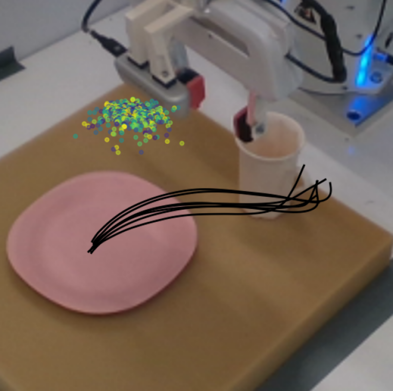
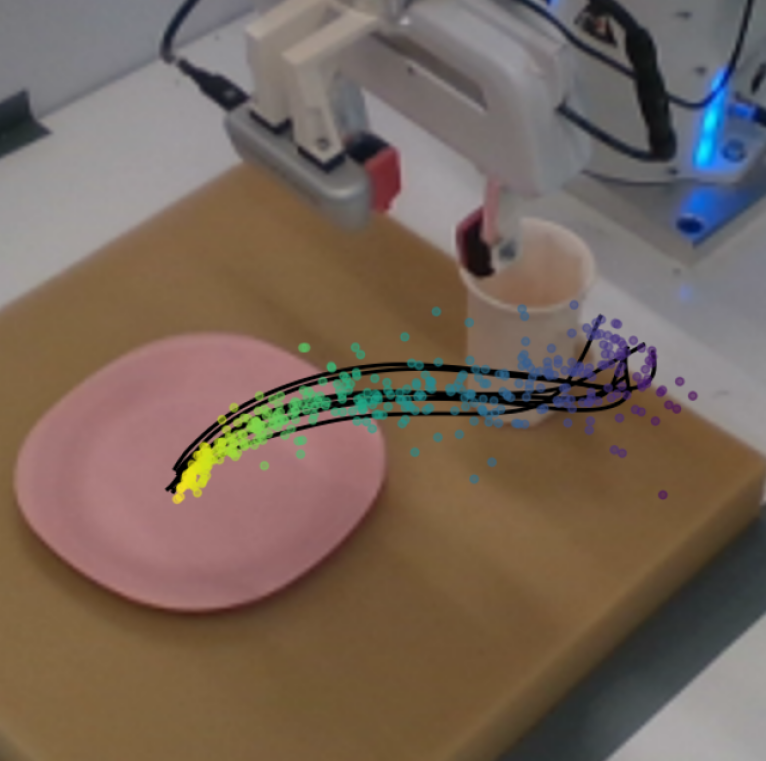
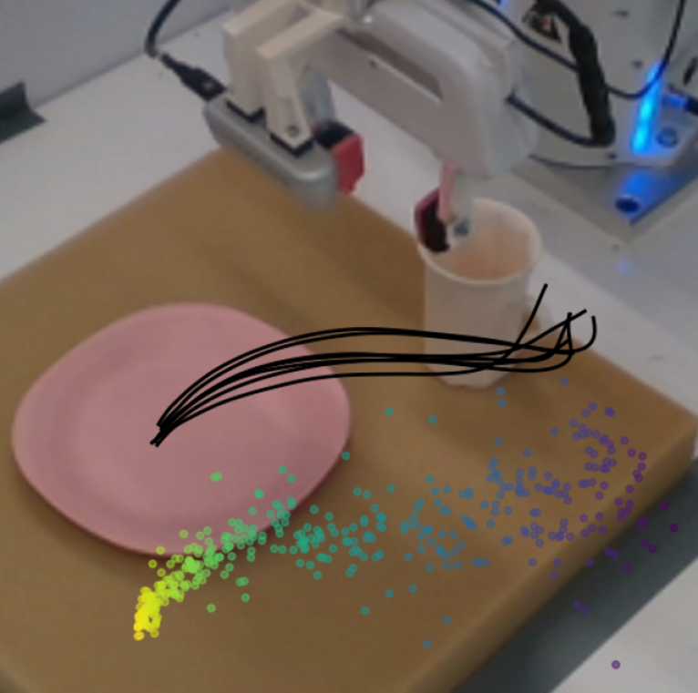
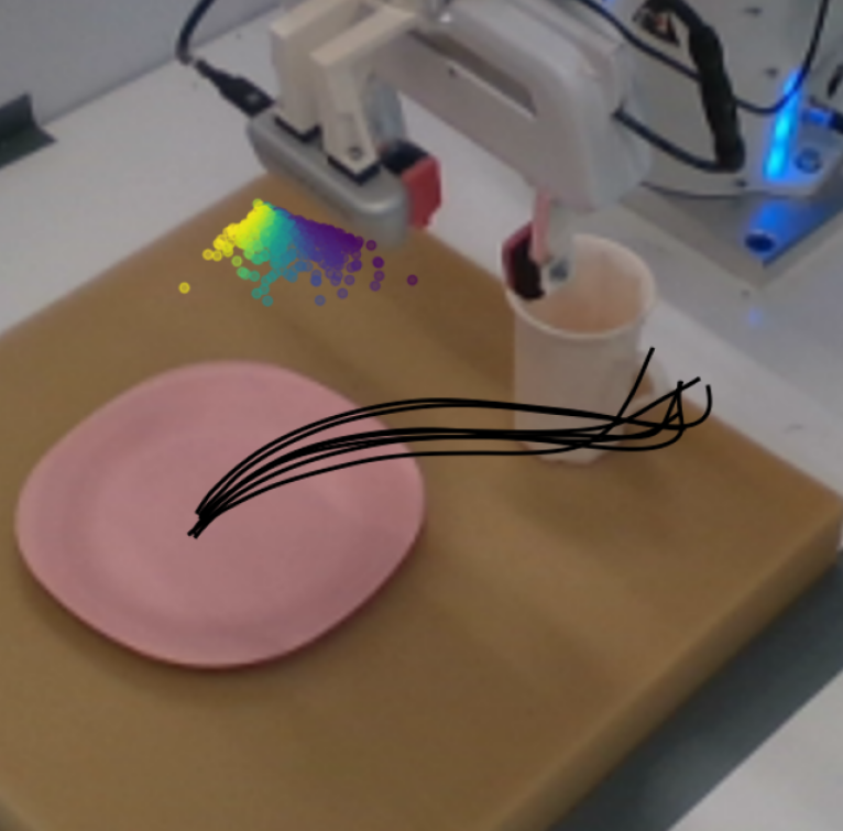

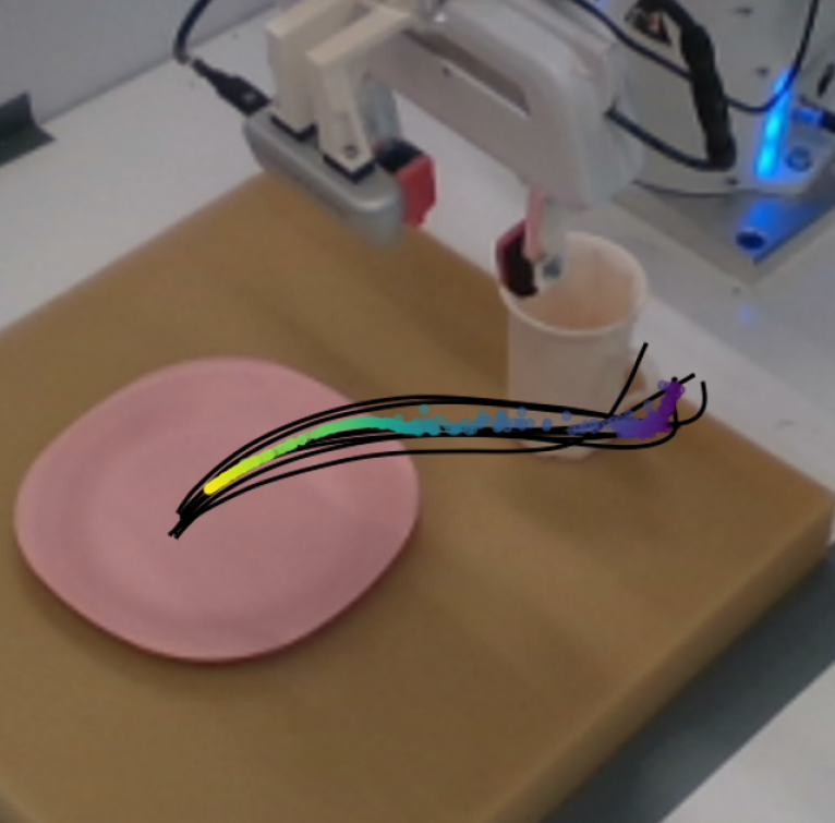
Figure 1:Flows of the RFMP (top) and SRFMP (bottom) at times t={0.0,1.0,1.5}. The policies are learned from pick-and-place demonstration (black) and conditioned on visual observations. Note that the flow of SRFMP is stable to the target distribution at t>1.0, enhancing the policy robustness and inference time.
图 1:RFMP(顶部)和 SRFMP(底部)在时间 t={0.0,1.0,1.5} 的流动。策略是从拾取和放置演示(黑色)中学习的,并以视觉观察为条件。请注意,SRFMP 的流动在 t>1.0 时对目标分布是稳定的,从而增强了策略的鲁棒性和推理时间。
To overcome these limitations, we propose to learn visuomotor robot skills via a Riemannian flow matching policy (RFMP). Compared to DP, RFMP builds on another kind of generative model: Flow Matching (FM) [15, 16]. Intuitively, FM gradually transforms a simple prior distribution into a complex target distribution via a vector field, which is represented by a simple function. The beauty of FM lies in its simplicity, as the resulting flow, defined by an ordinary differential equation (ODE), is much easier to train and much faster to evaluate compared to the stochastic differential equations of diffusion models. However, as many visuomotor policies are represented in the robot’s operational space, action representations must include both end-effector position and orientation. Thus, the policy must consider that orientations lie on either the 𝒮3 hypersphere or the SO(3) Lie group, depending on the specific parametrization. To properly handle such data, we leverage Riemannian flow matching (RFM) [16], an extension of flow matching that accounts for the geometric constraints of data lying on Riemannian manifolds. In our previous work [17], we introduced the idea of leveraging flow matching in robot imitation learning and presented RFMP, which capitalizes on the easy training and fast inference of FM methods to learn and synthesize end-effector pose trajectories. However, our initial evaluation was limited to simple proof-of-concept experiments on the LASA dataset [18].
为克服这些限制,我们提出通过黎曼流匹配策略(RFMP)学习视觉运动机器人技能。与 DP 相比,RFMP 建立在另一种生成模型:流匹配(FM)[15, 16]的基础上。直观地说,FM 通过向量场逐渐将简单的先验分布转变为复杂的目标分布,该向量场由一个简单函数表示。FM 的美在于其简单性,因为由常微分方程(ODE)定义的结果流相比扩散模型的随机微分方程更容易训练且评估速度更快。然而,由于许多视觉运动策略在机器人的操作空间中表示,动作表示必须包括末端执行器的位置和方向。因此,策略必须考虑到方向取决于特定参数化,位于 𝒮3 超球面或 SO(3) 李群上。为了正确处理这些数据,我们利用黎曼流匹配(RFM)[16],这是流匹配的扩展,考虑了位于黎曼流形上的数据的几何约束。 在我们之前的工作[17]中,我们引入了在机器人模仿学习中利用流匹配的想法,并提出了 RFMP,它利用 FM 方法的简单训练和快速推理来学习和合成末端执行器姿态轨迹。然而,我们的初步评估仅限于在 LASA 数据集[18]上的简单概念验证实验。
In this paper, we demonstrate the effectiveness of RFMP to learn complex real-world visuomotor policies and present a systematic evaluation of the performance of RFMP on both simulated and real-world manipulation tasks. Moreover, we propose Stable Riemannian Flow Matching Policy (SRFMP) to enhance the robustness of RFMP (see Figure 1). SRFMP builds on stable flow matching (SFM) [19, 20], which leverages LaSalle’s invariance principle [21] to equip the dynamics of FM with stability to the support of the target distribution. Unlike SFM, which is limited to Euclidean spaces, SRFMP generalizes this concept to Riemannian manifolds, guaranteeing the stability of the RFM dynamics to the support of a Riemannian target distribution. We systematically evaluate RFMP and SRFMP across 8 tasks in both simulation and real-world settings, with policies conditioned on both state and visual observations. Our experiments demonstrate that RFMP and SRFMP inherit the advantages from FM models, achieving comparable performance to DP with fewer evaluation steps (i.e., faster inference) and significantly shorter training times. Moreover, our models achieve competitive performance compared to CP [3] on several simulated tasks. Notably, SRFMP requires fewer ODE steps than RFMP to achieve an equivalent performance, resulting in even faster inference times.
在本文中,我们展示了 RFMP 在学习复杂的现实世界视觉运动策略方面的有效性,并系统地评估了 RFMP 在模拟和现实世界操作任务中的性能。此外,我们提出了稳定黎曼流匹配策略(SRFMP),以增强 RFMP 的鲁棒性(见图 1)。SRFMP 建立在稳定流匹配(SFM)[19, 20]的基础上,利用 LaSalle 的不变性原理[21]使 FM 的动态对目标分布的支持具有稳定性。与仅限于欧几里得空间的 SFM 不同,SRFMP 将这一概念推广到黎曼流形,保证了 RFM 动态对黎曼目标分布支持的稳定性。我们系统地评估了 RFMP 和 SRFMP 在模拟和现实世界环境中的 8 个任务,策略基于状态和视觉观测条件。我们的实验表明,RFMP 和 SRFMP 继承了 FM 模型的优势,以更少的评估步骤(即更快的推理)和显著更短的训练时间实现了与 DP 相当的性能。 此外,我们的模型在多个模拟任务中表现出与 CP [3]相当的竞争力。值得注意的是,SRFMP 比 RFMP 需要更少的 ODE 步骤即可达到相同的性能,从而实现更快的推理时间。
In summary, beyond demonstrating the effectiveness of our early work on simulated and real robotic tasks, the main contributions of this article are threefold: (1) We introduce Stable Riemannian Flow Matching (SRFM) as an extension of SFM [20] to incorporate stability into RFM; (2) We propose stable Riemannian flow matching policy (SRFMP), which combines the easy training and fast inference of RFMP with stability guarantees to Riemannian target action distribution; (3) We systematically evaluate both RFMP and SRFMP across 8 tasks from simulated benchmarks and real settings. Supplementary material is available on the paper website https://sites.google.com/view/rfmp.
总之,除了展示我们在模拟和真实机器人任务上的早期工作的有效性外,本文的主要贡献有三点:(1) 我们引入了稳定黎曼流匹配 (SRFM),作为 SFM [20] 的扩展,将稳定性纳入 RFM;(2) 我们提出了稳定黎曼流匹配策略 (SRFMP),它结合了 RFMP 的易训练和快速推理,并对黎曼目标动作分布提供稳定性保证;(3) 我们系统地评估了 RFMP 和 SRFMP 在模拟基准和真实环境中的 8 个任务。补充材料可在论文网站 https://sites.google.com/view/rfmp 上找到。
IIRelated work II 相关工作
As the literature on robot policy learning is arguably vast, we here focus on approaches that design robot policies based on flow-based generative models.
由于机器人策略学习的文献可以说是非常广泛的,我们在这里重点关注基于流生成模型设计机器人策略的方法。
Normalizing Flows are arguably the first broadly-used generative models in robot policy learning [22]. They were commonly employed as diffeomorphisms for learning stable dynamical systems in Euclidean spaces [23, 24, 25], with extensions to Lie groups [26] and Riemannian manifolds [27], similarly addressed in this paper. The main drawback of normalizing flows is their slow training, as the associated ODE needs to be integrated to calculate the log-likelihood of the model. Moreover, none of the aforementioned works learned sensorimotor policies based on visual observations via imitation learning.
归一化流可以说是机器人策略学习中最广泛使用的生成模型 [22]。它们通常被用作微分同胚,用于在欧几里得空间中学习稳定的动力系统 [23, 24, 25],并扩展到李群 [26] 和黎曼流形 [27],本文也同样涉及。归一化流的主要缺点是训练速度慢,因为需要积分相关的常微分方程来计算模型的对数似然。此外,上述工作中没有一个是通过模仿学习基于视觉观察来学习传感运动策略的。
Diffusion Models [28] recently became state-of-art in imitation learning because of their ability to learn multi-modal and high-dimensional action distributions. They have been primarily employed to learn motion planners [29], and complex control policies [2, 30, 4]. Recent extensions consider to use 3D visual representations from sparse point clouds [6], and to employ equivariant networks for learning policies that, by design, are invariant to changes in scale, rotation, and translation [7]. However, a major drawback of diffusion models is their slow inference process. In [2], DP requires 10 to 100 denoising steps, i.e., 0.1 to 1 second on a standard GPU, to generate each action. Consistency models (CM) [31] arise as a potential solution to overcome this drawback [3, 32, 33]. CM distills a student model from a pretrained diffusion model (i.e., a teacher), enabling faster inference by establishing direct connections between points along the probability path. Nevertheless, this sequential training process increases the overall complexity and time of the whole training phase.
扩散模型 [28] 最近在模仿学习中成为最先进的技术,因为它们能够学习多模态和高维动作分布。它们主要用于学习运动规划器 [29] 和复杂的控制策略 [2, 30, 4]。最近的扩展考虑使用稀疏点云的 3D 视觉表示 [6],并采用等变网络来学习在设计上对尺度、旋转和平移变化不变的策略 [7]。然而,扩散模型的一个主要缺点是它们的推理过程缓慢。在 [2] 中,DP 需要 10 到 100 的去噪步骤,即在标准 GPU 上生成每个动作需要 0.1 到 1 秒。一致性模型 (CM) [31] 出现作为克服这一缺点的潜在解决方案 [3, 32, 33]。CM 从预训练的扩散模型(即教师)中提取学生模型,通过在概率路径上的点之间建立直接连接,实现更快的推理。然而,这种顺序训练过程增加了整个训练阶段的整体复杂性和时间。
Flow Matching [15] essentially trains a normalizing flow by regressing a conditional vector field instead of maximizing the likelihood of the model, thus avoiding to simulate the ODE of the flow. This leads to a significantly simplified training procedure compared to classical normalizing flows. Moreover, FM builds on simpler probability transfer paths than diffusion models, thus facilitating faster inference. Tong et al. [34] showed that several types of FM models can be obtained according to the choice of conditional vector field and source distributions, some of them leading to straighter probability paths, which ultimately result in faster inference. Rectified flows [35] is a similar simulation-free approach that designs the vector field by regressing against straight-line paths, thus speeding up inference. Note that rectified flows are a special case of FM, in which a Dirac distribution is associated to the probability path [34]. Due to their easy training and fast inference, FM models quickly became one of the de-facto generative models in machine learning and have been employed in a plethora of different applications [36, 37, 38, 39, 40, 41].
流匹配 [15] 本质上是通过回归条件向量场来训练归一化流,而不是最大化模型的似然性,从而避免模拟流的 ODE。这导致与经典归一化流相比,训练过程显著简化。此外,FM 基于比扩散模型更简单的概率传输路径,从而促进更快的推理。Tong 等人 [34] 表明,根据条件向量场和源分布的选择,可以获得几种类型的 FM 模型,其中一些导致更直的概率路径,最终导致更快的推理。校正流 [35] 是一种类似的无模拟方法,通过回归直线路径来设计向量场,从而加快推理速度。请注意,校正流是 FM 的一种特殊情况,其中 Dirac 分布与概率路径相关联 [34]。由于其易于训练和快速推理,FM 模型迅速成为机器学习中事实上的生成模型,并已应用于大量不同的应用 [36, 37, 38, 39, 40, 41]。
In our previous work [17], we proposed to leverage RFM to learn sensorimotor robot policies represented by end-effector pose trajectories on Riemannian manifolds. Building on a similar idea, subsequent works have used FM along with an equivariant transformer to learn SE(3)-equivariant policies [42], for multi-support manipulation tasks with a humanoid robot [43], and for point-cloud-based robot imitation learning [44]. In this paper, we build upon our previous work, Riemannian Flow Matching Policy (RFMP), to enable the learning of complex visuomotor policies on Riemannian manifolds. Unlike the aforementioned approaches, our work focuses on providing a fast and robust RFMP inference process. We achieve this by constructing the FM vector field using LaSalle’s invariance principle, which not only enhances inference robustness with stability guarantees but also preserves the easy training and fast inference capabilities of RFMP.
在我们之前的工作[17]中,我们提出利用 RFM 来学习由末端执行器姿态轨迹表示的黎曼流形上的传感运动机器人策略。基于类似的想法,后续工作使用 FM 和等变变压器来学习 SE(3) -等变策略[42],用于多支撑操作任务的人形机器人[43],以及基于点云的机器人模仿学习[44]。在本文中,我们基于之前的工作,黎曼流匹配策略(RFMP),以实现黎曼流形上复杂视觉运动策略的学习。与上述方法不同,我们的工作重点是提供快速且稳健的 RFMP 推理过程。我们通过使用 LaSalle 不变性原理构建 FM 向量场来实现这一点,这不仅增强了推理的稳健性并提供稳定性保证,还保留了 RFMP 的易训练和快速推理能力。
IIIBackground III 背景
In this section, we provide a short background on Riemannian manifolds, and an overview of the flow matching framework with its extension to Riemannian manifolds.
在本节中,我们提供了黎曼流形的简短背景,并概述了流匹配框架及其在黎曼流形上的扩展。
III-ARiemannian Manifolds
III-A 黎曼流形
A smooth manifold ℳ can be intuitively understood as a d-dimensional surface that locally, but not globally, resembles the Euclidean space ℝd [45, 46]. The geometric structure of the manifold is described via the so-called charts, which are diffeomorphic maps between parts of ℳ and ℝ. The collection of these charts is called an atlas. The smooth structure of ℳ allows us to compute derivatives of curves on the manifolds, which are tangent vectors to ℳ at a given point 𝒙. For each point 𝒙∈ℳ, the set of tangent vectors 𝒖 of all curves that pass through 𝒙 forms the tangent space 𝒯𝒙ℳ. The tangent space spans a d-dimensional affine subspace of ℝd, where d is the manifold dimension. The collections of all tangent spaces of ℳ forms the tangent bundle 𝒯ℳ=⋃𝒙∈ℳ{(𝒙,𝒖)|𝒖∈𝒯𝒙ℳ}, which can be thought as the union of all tangent spaces paired with their corresponding points on ℳ.
光滑流形 ℳ 可以直观地理解为一个 d 维的曲面,在局部上但不是整体上类似于欧几里得空间 ℝd [45, 46]。流形的几何结构通过所谓的图来描述,这些图是 ℳ 和 ℝ 之间的微分同胚映射。这些图的集合称为图集。 ℳ 的光滑结构允许我们计算流形上曲线的导数,这些导数是给定点 𝒙 处 ℳ 的切向量。对于每个点 𝒙∈ℳ ,所有通过 𝒙 的曲线的切向量 𝒖 的集合形成切空间 𝒯𝒙ℳ 。切空间跨越 ℝd 的一个 d 维仿射子空间,其中 d 是流形维度。所有 ℳ 的切空间的集合形成切丛 𝒯ℳ=⋃𝒙∈ℳ{(𝒙,𝒖)|𝒖∈𝒯𝒙ℳ} ,可以认为是所有切空间与其在 ℳ 上对应点的并集。
Riemannian manifolds are smooth manifolds equipped with a smoothly-varying metric g, which is a family of inner products g𝒙:𝒯𝒙ℳ×𝒯𝒙ℳ→ℝ. The norm associated with the metric is denoted as ‖𝒗‖g𝒙 with 𝒗∈𝒯𝒙ℳ, and the distance between two vectors 𝒖,𝒗∈𝒯𝒙ℳ is defined as the norm ‖𝒖−𝒗‖g𝒙. With this metric, we can then define the length of curves on ℳ. The shortest curve on ℳ connecting any two points 𝒙,𝒚∈ℳ is called a geodesic. Intuitively, geodesics can be seen as the generalization of straight lines to Riemannian manifolds. To operate with Riemannian manifolds, a common way is to exploit its Euclidean tangent spaces 𝒯𝒙ℳ and back-and-forth maps between ℳ and 𝒯𝒙ℳ, i.e., the exponential and logarithmic maps. Specifically, the exponential map Exp𝒙(𝒖):𝒯𝒙ℳ→ℳ maps a point 𝒖 on the tangent space of 𝒙 to a point 𝒚∈ℳ, so that the geodesic distance between 𝒚=Exp𝒙(𝒖) and 𝒙 satisfies dg(𝒙,𝒚)=‖𝒖‖g𝒙. The inverse operation is the logarithmic map Log𝒙(𝒚):ℳ→𝒯𝒙ℳ, which projects a point 𝒚∈ℳ to the tangent space 𝒯𝒙ℳ of 𝒙. Finally, when optimizing functions of manifold-valued parameters, we need to compute the Riemannian gradient. Specifically, the Riemannian gradient of a scalar function f:ℳ→ℝ at 𝒙∈ℳ is a vector in the tangent space 𝒯𝒙ℳ [47, 48]. It is obtained via the identification ℒ𝒖f(𝒙)=〈∇𝒙f(𝒙),𝒖〉𝒙, where ℒ𝒖f(𝒙) denotes the directional derivative of f in the direction 𝒖∈𝒯𝒙ℳ, and 〈⋅,⋅〉𝒙 is the Riemannian inner product on 𝒯𝒙ℳ.
黎曼流形是配备有平滑变化度量的光滑流形 g ,这是一族内积 g𝒙:𝒯𝒙ℳ×𝒯𝒙ℳ→ℝ 。与度量相关的范数表示为 ‖𝒗‖g𝒙 ,并且两个向量之间的距离 𝒖,𝒗∈𝒯𝒙ℳ 定义为范数 ‖𝒖−𝒗‖g𝒙 。通过这个度量,我们可以定义曲线在 ℳ 上的长度。连接任意两点 𝒙,𝒚∈ℳ 的最短曲线 ℳ 称为测地线。从直观上看,测地线可以看作是直线在黎曼流形上的推广。操作黎曼流形的一种常见方法是利用其欧几里得切空间 𝒯𝒙ℳ 及其之间的往返映射 ℳ 和 𝒯𝒙ℳ ,即指数映射和对数映射。具体来说,指数映射 Exp𝒙(𝒖):𝒯𝒙ℳ→ℳ 将 𝒙 的切空间上的一点 𝒖 映射到一点 𝒚∈ℳ ,使得 𝒚=Exp𝒙(𝒖) 和 𝒙 之间的测地距离满足 dg(𝒙,𝒚)=‖𝒖‖g𝒙 。逆操作是对数映射 Log𝒙(𝒚):ℳ→𝒯𝒙ℳ ,它将一点 𝒚∈ℳ 投影到 𝒙 的切空间 𝒯𝒙ℳ 。最后,在优化流形值参数的函数时,我们需要计算黎曼梯度。 具体来说,标量函数 f:ℳ→ℝ 在 𝒙∈ℳ 处的黎曼梯度是切空间 𝒯𝒙ℳ 中的一个向量[47, 48]。它是通过识别 ℒ𝒖f(𝒙)=〈∇𝒙f(𝒙),𝒖〉𝒙 获得的,其中 ℒ𝒖f(𝒙) 表示 f 在方向 𝒖∈𝒯𝒙ℳ 上的方向导数, 〈⋅,⋅〉𝒙 是 𝒯𝒙ℳ 上的黎曼内积。
III-BFlow Matching III-B 流匹配
Continuous normalizing flows (CNF) [49] form a class of deep generative models that transform a simple probability distribution into a more complex one. The continuous transformation of the samples is parametrized by an ODE, which describes the flow of the samples over time. Training CNF is achieved via maximum likelihood estimation, and thus involves solving (a.k.a. simulating) inverse ODEs, which is computationally expensive. Instead, flow matching (FM) [15] is a simulation-free generative model that efficiently trains CNF by directly mimicking a target vector field.
连续归一化流(CNF)[49] 形成了一类深度生成模型,将简单的概率分布转化为更复杂的分布。样本的连续变换由一个常微分方程(ODE)参数化,该方程描述了样本随时间的流动。通过最大似然估计来训练 CNF,因此涉及求解(即模拟)逆 ODE,这在计算上是昂贵的。相反,流匹配(FM)[15] 是一种无模拟生成模型,通过直接模仿目标向量场来高效地训练 CNF。
III-B1Euclidean Flow Matching
III-B1 欧几里得流匹配
FM [15] reshapes a simple prior distribution p into a (more complicated) target distribution q via a probability density path pt that satisfies p0=p and p1=q. The path pt is generated by push-forwarding p0 along a flow ψt as,
FM [ 15] 将一个简单的先验分布 p 重新塑造成一个(更复杂的)目标分布 q ,通过满足 p0=p 和 p1=q 的概率密度路径 pt 。路径 pt 是通过沿着流 ψt 推送 p0 生成的,
| pt=[ψt]∗p0, | (1) |
where the push-forward operator ∗ is defined as,
其中推前算子 ∗ 定义为,
| [ψt]∗p0(𝒙)=p0(ψt−1(𝒙))det(∂ψt−1(𝒙)∂𝒙). | (2) |
The flow ψt(𝒙) is defined via a vector field ut:[0,1]×ℝd→ℝd by solving the ODE,
流 ψt(𝒙) 通过求解 ODE 由向量场 ut:[0,1]×ℝd→ℝd 定义
| dψt(𝒙)dt=ut(ψt(𝒙)),withψ0(𝒙)=𝒙. | (3) |
Assuming that both the vector field ut(𝒙) and probability density path pt are known, one can regress a parametrized vector field vt(𝒙;𝜽):[0,1]×ℝd→ℝd to some target vector field ut, which leads to the FM loss function,
假设已知向量场 ut(𝒙) 和概率密度路径 pt ,可以回归参数化向量场 vt(𝒙;𝜽):[0,1]×ℝd→ℝd 到某个目标向量场 ut ,这将导致 FM 损失函数,
| ℓFM(𝜽)=𝔼t,pt(𝒙)‖vt(𝒙;𝜽)−ut(𝒙)‖22, | (4) |
where 𝜽 are the learnable parameters, t∼𝒰[0,1], and 𝒙∼pt(𝒙). However, the loss (4) is intractable since we actually do not have prior knowledge about ut and pt. Instead, Lipman et al. [15] proposed to learn a conditional vector field ut(𝒙|𝒙1) with 𝒙1 as a conditioning variable. This conditional vector field generates the conditional probability density path pt(𝒙|𝒙1), which is related to the marginal probability path via pt(𝒙)=∫pt(𝒙|𝒙1)q(𝒙1)𝑑𝒙1, with q being the unknown data distribution. After reparametrization, this leads to the tractable conditional flow matching (CFM) loss function,
其中 𝜽 是可学习的参数, t∼𝒰[0,1] 和 𝒙∼pt(𝒙) 。然而,损失函数 (4) 是不可解的,因为我们实际上没有关于 ut 和 pt 的先验知识。相反,Lipman 等人 [15] 提出了学习一个以 𝒙1 作为条件变量的条件向量场 ut(𝒙|𝒙1) 。这个条件向量场生成了条件概率密度路径 pt(𝒙|𝒙1) ,它通过 pt(𝒙)=∫pt(𝒙|𝒙1)q(𝒙1)𝑑𝒙1 与边际概率路径相关,其中 q 是未知的数据分布。重新参数化后,这导致了可解的条件流匹配 (CFM) 损失函数。
| ℓCFM(𝜽)=𝔼t,q(𝒙1),p(𝒙0)∥vt(𝒙t;𝜽)−ut(𝒙t|𝒙1)∥22, | (5) |
where 𝒙t=ψt(𝒙0|𝒙1) denotes the conditional flow. Note that optimizing the CFM loss (5) is equivalent to optimizing the FM loss (4) as they have identical gradients [15]. The problem therefore boils down to design a conditional vector field ut(𝒙t|𝒙1) that generates a probability path pt satisfying the boundary conditions p0=p, q=p1. Intuitively, ut(𝒙t|𝒙1) should move a randomly-sampled point at t=0 to a datapoint at t=1. Lipman et al. [15] proposed the Gaussian CFM, which defines a probability path from a zero-mean normal distribution to a Gaussian distribution centered at 𝒙1 via the conditional vector field,
其中 𝒙t=ψt(𝒙0|𝒙1) 表示条件流。请注意,优化 CFM 损失 (5) 等同于优化 FM 损失 (4),因为它们具有相同的梯度 [15]。因此,问题归结为设计一个条件向量场 ut(𝒙t|𝒙1) ,该向量场生成满足边界条件 p0=p , q=p1 的概率路径 pt 。直观地, ut(𝒙t|𝒙1) 应该将 t=0 的随机采样点移动到 t=1 的数据点。Lipman 等人 [15] 提出了高斯 CFM,它通过条件向量场定义了从零均值正态分布到以 𝒙1 为中心的高斯分布的概率路径。
| ut(𝒙t|𝒙1)=𝒙1−(1−σ)𝒙0, | (6) |
which leads to the flow 𝒙t=ψt(𝒙0|𝒙1)=(1−(1−σ)t)𝒙0+t𝒙1. Note that a more general version of CFM is proposed by Tong et al. [34].
这导致了流 𝒙t=ψt(𝒙0|𝒙1)=(1−(1−σ)t)𝒙0+t𝒙1 。请注意,更通用的 CFM 版本由 Tong 等人提出[34]。
Finally, the inference process of CFM is straightforward and consists of the following steps: (1) Get a sample from p0; and (2) Query the learned vector field vt(𝒙;𝜽) to solve the ODE (3) with off-the-shelf solvers, e.g., based on the Euler method [50].
最后,CFM 的推理过程很简单,包括以下步骤:(1) 从 p0 获取样本;(2) 查询学习到的向量场 vt(𝒙;𝜽) 以使用现成的求解器(例如基于欧拉方法 [50])求解 ODE (3)。
III-B2Riemannian Flow Matching
III-B2 黎曼流匹配
In many robotics settings, data lies on Riemannian manifolds [51, 52]. For example, various tasks involve the rotation of the robot’s end-effector. Therefore, the corresponding part of the state representation lies either on the Riemannian hypersphere 𝒮3 or the SO(3) group, depending on the choice of parametrization. To guarantee that the FM generative process satisfies manifold constraints, Chen and Lipman [16] extended CFM to Riemannian manifolds. The Riemannian conditional flow matching (RCFM) considers that the flow ψt evolves on a Riemannian manifold ℳ. Thus, for each point 𝒙∈ℳ, the vector field associated to the flow ψt at this point lies on the tangent space of 𝒙, i.e., ut(𝒙)∈𝒯𝒙ℳ. The RCFM loss function resembles that of the CFM model but it is computed with respect to the Riemannian metric g𝒙 as follows,
在许多机器人设置中,数据位于黎曼流形上 [51, 52]。例如,各种任务涉及机器人末端执行器的旋转。因此,状态表示的相应部分位于黎曼超球面 𝒮3 或 SO(3) 群上,具体取决于参数化的选择。为了保证 FM 生成过程满足流形约束,Chen 和 Lipman [16] 将 CFM 扩展到黎曼流形。黎曼条件流匹配 (RCFM) 认为流 ψt 在黎曼流形 ℳ 上演变。因此,对于每个点 𝒙∈ℳ ,与该点处的流 ψt 相关的矢量场位于 𝒙 的切空间上,即 ut(𝒙)∈𝒯𝒙ℳ 。RCFM 损失函数类似于 CFM 模型,但它是相对于黎曼度量 g𝒙 计算的,如下所示,
| ℓRCFM=𝔼t,q(𝒙1),p(𝒙0)∥vt(𝒙t;𝜽)−ut(𝒙t|𝒙1)∥g𝒙t2. | (7) |
As in the Euclidean case, we need to design the flow ψt, its corresponding conditional vector field ut(𝒙t|𝒙1), and choose the base distribution. Following [16, 36], the most straightforward strategy is to exploit geodesic paths to design the flow ψt. For simple Riemannian manifolds such as the hypersphere, the hyperbolic manifold, and some matrix Lie groups, geodesics can be computed via closed-form solutions. We can then leverage the geodesic flow given by,
与欧几里得情况一样,我们需要设计流 ψt ,其对应的条件向量场 ut(𝒙t|𝒙1) ,并选择基分布。根据[16, 36],最直接的策略是利用测地路径来设计流 ψt 。对于简单的黎曼流形,如超球面、双曲流形和一些矩阵李群,测地线可以通过闭式解计算。然后我们可以利用给定的测地流,
| 𝒙t=Exp𝒙1(tLog𝒙1(𝒙0)),t∈[0,1]. | (8) |
The conditional vector field can then be calculated as the time derivative of 𝒙t, i.e., ut(𝒙t|𝒙1)=𝒙˙t. Notice that ut boils down to the conditional vector field (6) with σ=0 when ℳ=ℝd. Chen and Lipman [16] also provide a general formulation of ut(𝒙t|𝒙1) for cases where closed-form geodesics are not available. The prior distribution p0 can be chosen as a uniform distribution on the manifold [36, 16], or as a Riemannian [53] or wrapped Gaussian [16, 54] distribution on ℳ. During inference, we solve the corresponding RCFM’s ODE on the Riemannian manifold ℳ via projection-based methods. Specifically, at each step, the integration is performed in the tangent space 𝒯𝒙ℳ and the resulting vector is projected onto the Riemannian manifold ℳ with the exponential map.
条件向量场可以计算为 𝒙t 的时间导数,即 ut(𝒙t|𝒙1)=𝒙˙t 。注意,当 ℳ=ℝd 时, ut 简化为具有 σ=0 的条件向量场(6)。Chen 和 Lipman [16]还提供了 ut(𝒙t|𝒙1) 的一般公式,用于没有闭形式测地线的情况。先验分布 p0 可以选择为流形上的均匀分布[36, 16],或 ℳ 上的黎曼[53]或包裹高斯[16, 54]分布。在推理过程中,我们通过基于投影的方法在黎曼流形 ℳ 上求解相应的 RCFM 的 ODE。具体来说,在每一步中,积分在切空间 𝒯𝒙ℳ 中进行,结果向量通过指数映射投影到黎曼流形 ℳ 上。
III-CFlow Matching vs. Diffusion and Consistency Models
III-C 流匹配与扩散和一致性模型
Diffusion Policy (DP) [2] is primarily trained based on DDPM [12], which performs iterative denoising from an initial noise sample 𝒙K, where K denotes the total number of denoising steps. The denoising process follows,
扩散策略 (DP) [2] 主要基于 DDPM [12] 进行训练,DDPM 从初始噪声样本 𝒙K 进行迭代去噪,其中 K 表示去噪步骤的总数。去噪过程如下,
| 𝒙k−1=αt(𝒙k−γϵ𝜽(𝒙k,k)+𝒩(0,σ2𝑰)), | (9) |
where α, γ and σ constitute the noise schedule that governs the denoising process, and ϵθ(𝒙k,k) is the noise prediction network that infers the noise at the k-th denoising step. The final sample 𝒙0 is the noise-free target output. The equivalent inference process in FM is governed by,
其中 α 、 γ 和 σ 构成了控制去噪过程的噪声计划, ϵθ(𝒙k,k) 是在第 k 个去噪步骤中推断噪声的噪声预测网络。最终样本 𝒙0 是无噪声的目标输出。FM 中的等效推理过程由以下内容控制,
| dψt(𝒙)dt=vt(ψt(𝒙);𝜽),withψ0(𝒙)=𝒙, | (10) |
where vt(ψt(𝒙);𝜽) is the learned vector field that mimics the target forward process (6). Two key differences can be identified: (1) FM requires to solve a simple ODE, and (2) The FM vector field induces straighter paths. Importantly, the DP denoising framework limits its inference efficiency, particularly in scenarios requiring faster predictions.
其中 vt(ψt(𝒙);𝜽) 是模拟目标前向过程(6)的学习向量场。可以确定两个关键区别:(1)FM 需要解决一个简单的 ODE,(2)FM 向量场引导更直的路径。重要的是,DP 去噪框架限制了其推理效率,特别是在需要更快预测的情况下。
Consistency Policy (CP) [3] aims to speed up the inference process of DP by leveraging a consistency model that distills the DP as a teacher model. While CP adopts a similar denoising mechanism as DP, it enhances the process by incorporating both the current denoising step k and the target denoising step t as inputs to the denoising network, formalized as ϵθ(𝒙k,k,t). However, CP involves a two-stage training process. First, a DP teacher policy is trained. Next, a student policy is trained to mimic the denoising process of the teacher policy. This approach enables CP to achieve faster and more efficient inference while retaining the performance of its teacher model, at the cost of a more complex training process. In contrast, FM training is simulation-free, and features a single-phase training with a simple loss function.
一致性策略 (CP) [3] 旨在通过利用一致性模型将 DP 作为教师模型来加速 DP 的推理过程。虽然 CP 采用了与 DP 类似的去噪机制,但它通过将当前去噪步骤 k 和目标去噪步骤 t 作为输入纳入去噪网络来增强该过程,形式化为 ϵθ(𝒙k,k,t) 。然而,CP 涉及两个阶段的训练过程。首先,训练 DP 教师策略。接下来,训练学生策略以模仿教师策略的去噪过程。这种方法使 CP 能够在保持其教师模型性能的同时实现更快、更高效的推理,但代价是更复杂的训练过程。相比之下,FM 训练是无仿真的,并且具有简单损失函数的单阶段训练。
IVFast and Robust RFMP
IV 快速且稳健的 RFMP
Our goal is to leverage the RCFM framework to learn a parameterized policy π𝜽(𝒂|𝒐) that adheres to the target (expert) policy πe(𝒂|𝒐), which generates a set of N demonstrations Dn={𝒐s,𝒂s}s=1T, where 𝒐 denotes an observation, 𝒂 represents the corresponding action, and T denotes the length of n-th trajectory. In this section, we first introduce Riemaniann flow matching polices (RFMP) that leverage RCFM to achieve easy training and fast inference. Second, we propose Stable RFMP (SRFMP), an extension of RFMP that enhances its robustness and inference speed through stability to the target distribution.
我们的目标是利用 RCFM 框架学习一个参数化策略 π𝜽(𝒂|𝒐) ,该策略遵循目标(专家)策略 πe(𝒂|𝒐) ,生成一组 N 演示 Dn={𝒐s,𝒂s}s=1T ,其中 𝒐 表示观察, 𝒂 表示相应的动作, T 表示 n -th 轨迹的长度。在本节中,我们首先介绍利用 RCFM 实现轻松训练和快速推理的黎曼流匹配策略(RFMP)。其次,我们提出了稳定 RFMP(SRFMP),这是 RFMP 的扩展,通过对目标分布的稳定性增强其鲁棒性和推理速度。
IV-ARiemannian Flow Matching Policy
IV-A 黎曼流匹配策略
RFMP adapts RCFM to visuomotor robot policies by learning an observation-conditioned vector field ut(𝒂|𝒐). Similar to DP [2], RFMP employs a receding horizon control strategy [55], by predicting a sequence of actions over a prediction horizon Tp. This strategy aims at providing temporal consistency and smoothness on the predicted actions. This means that the predicted action horizon vector is constructed as 𝒂=[𝒂s,𝒂s+1,…,𝒂s+Tp], where 𝒂i is the action at time step i, and Tp is the action prediction horizon. This implies that all samples 𝒂1, drawn from the target distribution p1, have the form of the action horizon vector 𝒂. Moreover, we define the base distribution p0 such that samples 𝒂p0∼p0 are of the form 𝒂0=[𝒂b,…,𝒂b] with 𝒂b sampled from an auxiliary distribution b. This structure contributes to the smoothness of the predicted action vector 𝒂, as the flow of all its action components start from the same initial action 𝒂b.
RFMP 通过学习观察条件向量场 ut(𝒂|𝒐) 将 RCFM 适应于视觉运动机器人策略。类似于 DP [2],RFMP 采用递归视界控制策略[55],通过预测预测视界 Tp 上的一系列动作来实现。这种策略旨在提供预测动作的时间一致性和平滑性。这意味着预测动作视界向量被构建为 𝒂=[𝒂s,𝒂s+1,…,𝒂s+Tp] ,其中 𝒂i 是时间步 i 的动作, Tp 是动作预测视界。这意味着从目标分布 p1 中抽取的所有样本 𝒂1 都具有动作视界向量 𝒂 的形式。此外,我们定义了基分布 p0 ,使得样本 𝒂p0∼p0 具有 𝒂0=[𝒂b,…,𝒂b] 的形式,其中 𝒂b 从辅助分布 b 中抽取。这种结构有助于预测动作向量 𝒂 的平滑性,因为其所有动作组件的流动都从相同的初始动作 𝒂b 开始。
In contrast to the action horizon vector, the observation vector 𝒐 is not defined on a receding horizon but is constructed by randomly sampling only few observation vectors. Specifically, RFMP follows the sampling strategy proposed in [37] which uses: (1) A reference observation 𝒐s−1 at time step s−1; (2) A context observation 𝒐c randomly sampled from an observation window with horizon To, i.e., c is uniformly sampled from [s−To,s−2]; and (3) The time gap s−c between the context observation and reference observation. Therefore, the observation vector is defined as 𝒐=[𝒐s−1,𝒐c,s−c]. Notice that, when To=2, we disregard the time gap and the observation is 𝒐=[𝒐s−1,𝒐c]. The aforementioned strategy leads to the following RFMP loss function,
与动作视界向量相比,观测向量 𝒐 不是在回退视界上定义的,而是通过随机采样少量观测向量构建的。具体来说,RFMP 遵循[37]中提出的采样策略,该策略使用:(1)时间步 s−1 的参考观测 𝒐s−1 ;(2)从视界为 To 的观测窗口中随机采样的上下文观测 𝒐c ,即 c 从 [s−To,s−2] 中均匀采样;(3)上下文观测与参考观测之间的时间间隔 s−c 。因此,观测向量定义为 𝒐=[𝒐s−1,𝒐c,s−c] 。注意,当 To=2 时,我们忽略时间间隔,观测为 𝒐=[𝒐s−1,𝒐c] 。上述策略导致以下 RFMP 损失函数,
| ℓRFMP=𝔼t,q(𝒂1),p(𝒂0)∥vt(𝒂t|𝒐;𝜽)−ut(𝒂t|𝒂1)∥g𝒂t2. | (11) |
Algorithm 1 summarizes the training process of RFMP. Note that our RFMP inherits most of the training framework of RCFM, the main difference being that the vector field learned in RFMP is conditioned on the observation vector 𝒐.
算法 1 总结了 RFMP 的训练过程。请注意,我们的 RFMP 继承了 RCFM 的大部分训练框架,主要区别在于 RFMP 中学习的向量场是以观测向量 𝒐 为条件的。
初始参数 𝜽 ,先验和目标分布 p0 , p1 .
输出:学习到的向量场参数 𝜽 。
1 当终止条件不满足时 do
2 从均匀分布 𝒰[0,1] 中采样流时间步 t 。
3 样本噪声 𝒂0∼p0 .
4 联合采样动作序列 𝒂1∼p1 和相应的观测向量 𝒐 。
5 通过 RCFM 流形流 (8) 计算条件向量场 ut(𝒂t|𝒂1) 。
6 评估 ℓRFMP 如 (11) 中所示。
7 更新参数 𝜽 .
算法 1 RFMP 训练过程
After training RFMP, the inference process, which essentially queries the policy π𝜽(𝒂|𝒐), boils down to the following four steps: (1) Draw a sample 𝒂0 from the prior distribution p0; (2) Construct the observation vector 𝒐; (3) Employ an off-the-shelf ODE solver to integrate the learned vector field vt(𝒂|𝒐;𝜽) from 𝒂0 along the time interval t=[0,1], and get the generated action sequence 𝒂=[𝒂s,…,𝒂s+Tp]; (4) Execute the first Ta actions of the sequence 𝒂 with Ta≤Tp. This last step allows the robot to quickly react to environment changes, while still providing smooth predicted actions.
在训练 RFMP 之后,推理过程本质上是查询策略 π𝜽(𝒂|𝒐) ,归结为以下四个步骤:(1) 从先验分布 p0 中抽取样本 𝒂0 ;(2) 构建观测向量 𝒐 ;(3) 使用现成的 ODE 求解器从 𝒂0 沿时间间隔 t=[0,1] 积分学习的向量场 vt(𝒂|𝒐;𝜽) ,并获得生成的动作序列 𝒂=[𝒂s,…,𝒂s+Tp] ;(4) 使用 Ta≤Tp 执行序列 𝒂 的前 Ta 个动作。最后一步允许机器人快速对环境变化做出反应,同时仍然提供平滑的预测动作。
IV-BStable Riemannian Flow Matching Policy
IV-B 稳定黎曼流匹配策略
Both CFM and RCFM train and integrate the learned vector field vt(𝒙|𝜽) within the interval [0,1]. However, they do not guarantee that the flow converges stably to the target distribution at t=1. Besides, the associated vector field may even display strongly diverging behaviors when going beyond this upper boundary [20]. The aforementioned issues may arise due to numerical inaccuracies when training or integrating the vector field. To solve this problem, Sprague et al. [20] proposed Stable Autonomous Flow Matching (SFM) [20], which equips the dynamics of FM with stability to the support of the target distribution. Here, we propose to improve RFMP with SFM, which we generalize to the Riemannian case, in order to guarantee that the flow stabilizes to the target policy at t=1. Our experiments show that this approach not only enhances RFMP’s robustness but also further reduces inference time.
CFM 和 RCFM 都在区间 [0,1] 内训练和集成学习的向量场 vt(𝒙|𝜽) 。然而,它们并不能保证流在 t=1 处稳定地收敛到目标分布。此外,当超出此上边界时,相关向量场甚至可能表现出强烈的发散行为 [20]。上述问题可能是由于训练或集成向量场时的数值不准确所引起的。为了解决这个问题,Sprague 等人 [20] 提出了稳定自主流匹配 (SFM) [20],它为 FM 的动态提供了对目标分布支持的稳定性。在这里,我们提出用 SFM 改进 RFMP,并将其推广到黎曼情况,以保证流在 t=1 处稳定到目标策略。我们的实验表明,这种方法不仅增强了 RFMP 的鲁棒性,还进一步减少了推理时间。
IV-B1Stable Euclidean FMP
IV-B1 稳定欧几里得 FMP
We first summarize the Euclidean SFM [20], and then show how SFM can be integrated into RFMP. SFM leverages the stochastic LaSalle’s invariance principle [56, 57] — a criterion from control theory used to characterize the asymptotic stability of stochastic autonomous dynamical systems — to design a stable vector field u. Sprague et al. [20, Thm 3.8] adapts this principle to the FM setting as follows.
我们首先总结了欧几里得 SFM [20],然后展示如何将 SFM 集成到 RFMP 中。SFM 利用随机 LaSalle 不变性原理[56, 57]——一种控制理论中的标准,用于表征随机自治动力系统的渐近稳定性——来设计一个稳定的向量场 u 。Sprague 等人[20, Thm 3.8]将这一原理适应于 FM 设置如下。
Theorem 1. 定理 1.
(Stochastic LaSalle’s Invariance Principle) If there exists a time-independent vector field u, a flow ψ generated by u, and a positive scalar function H such that,
(随机 LaSalle 不变性原理) 如果存在一个时间不变的向量场 u ,由 u 生成的流 ψ ,以及一个正标量函数 H ,使得,
| ℒ𝒖H(𝒙)=∇𝒙H(𝒙)u(𝒙)≤0, | (12) |
where ℒ𝐮H(𝐱) is the directional derivative of the scalar function H in the direction 𝐮 and ∇𝐱H is the gradient of the function H, then,
其中 ℒ𝐮H(𝐱) 是标量函数 H 在方向 𝐮 上的方向导数, ∇𝐱H 是函数 H 的梯度,那么,
| limt→infψ(𝒙,t)∈{𝒙∈𝒳|ℒuH(𝒙)=0}, |
almost surely with 𝐱∼p(𝐱,0).
几乎肯定与 𝐱∼p(𝐱,0) 。
Intuitively, Theorem 1 provides conditions for convergence to an invariant set even when ℒuH(𝒙) is not strictly negative, therefore accounting for stochastic fluctuations in the system. Theorem 1 notably holds if u(𝒙) is a gradient field of H, i.e., if u(𝒙)=−∇𝒙H(𝒙)⊤. In this case, the problem of finding a stable vector field boils down to defining an appropriate scalar function H. As LaSalle’s invariance principle requires an autonomous, a.k.a time-independent, vector field, Sprague et al. [20] augment the FM state space 𝒙 with an additional dimension τ, called temperature or pseudo time, so that the SFM augmented state space becomes 𝝃=[𝒙,τ]. The pair (H,𝝃) is then defined so that it satisfies (12) as,
直观地说,定理 1 提供了收敛到不变集的条件,即使 ℒuH(𝒙) 不是严格负的,因此考虑了系统中的随机波动。如果 u(𝒙) 是 H 的梯度场,即如果 u(𝒙)=−∇𝒙H(𝒙)⊤ ,则定理 1 显著成立。在这种情况下,找到稳定向量场的问题归结为定义适当的标量函数 H 。由于 LaSalle 的不变性原理需要一个自主的,即时间不变的向量场,Sprague 等人[20]通过增加一个称为温度或伪时间的额外维度 τ 来扩展 FM 状态空间 𝒙 ,使得 SFM 扩展状态空间变为 𝝃=[𝒙,τ] 。然后定义对 (H,𝝃) 以满足(12),如下所示,
| H(𝝃|𝝃1)=12(𝝃−𝝃1)⊤𝑨(𝝃−𝝃1), | (13) |
| u(𝝃|𝝃1)=−∇𝝃H(𝝃|𝝃1)⊤=−𝑨(𝝃−𝝃1), | (14) |
where 𝑨 is a positive-define matrix. To simplify the calculation, 𝑨 is set as the diagonal matrix,
其中 𝑨 是正定矩阵。为了简化计算, 𝑨 被设为对角矩阵。
| 𝑨=[λ𝒙𝑰𝟎𝟎λτ], | (15) |
with λ𝒙,λτ∈ℝ. The vector field u and corresponding stable flow ψt are then given as,
与 λ𝒙,λτ∈ℝ 。然后给出向量场 u 及其对应的稳定流 ψt ,
| u(𝝃t|𝝃1)=[u𝒙(𝒙t|𝒙1)uτ(τt|τ1)]=[−λ𝒙(𝒙0−𝒙1)−λτ(τ0−τ1)], | (16) |
| ψt(𝝃0|𝝃1)=[ψt(𝒙0|𝒙1)ψt(τ0|τ1)]=[𝒙1+e−λ𝒙t(𝒙0−𝒙1)τ1+e−λτt(τ0−τ1)]. | (17) |
The parameters τ1 and τ0 define the range of the τ flow, while the parameters λ𝒙 and λτ determine its convergence. Specifically, the flow converges faster for higher values of λ𝒙 and λτ. Moreover, the ratio between λ𝒙/λτ determines the relative rate of convergence of the spatial and pseudo-time parts of the flow. We ablate the influence of λ𝒙 and λτ on SRFMP in Section V-B.
参数 τ1 和 τ0 定义了 τ 流的范围,而参数 λ𝒙 和 λτ 决定了其收敛性。具体来说,流在 λ𝒙 和 λτ 的值较高时收敛得更快。此外, λ𝒙/λτ 之间的比率决定了流的空间部分和伪时间部分的相对收敛速度。我们在第 V-B 节中消融了 λ𝒙 和 λτ 对 SRFMP 的影响。
We integrate SFM to RFMP by regressing an observation-conditioned vector field v(𝝃|𝒐;𝜽) to a stable target vector field u(𝝃t|𝝃1), where 𝝃=[𝒂s,…,𝒂s+Tp,τ] is the augmented prediction horizon vector, and 𝒐 is the observation vector.
我们通过将观测条件向量场 v(𝝃|𝒐;𝜽) 回归到稳定目标向量场 u(𝝃t|𝝃1) 来将 SFM 集成到 RFMP 中,其中 𝝃=[𝒂s,…,𝒂s+Tp,τ] 是增强的预测视界向量, 𝒐 是观测向量。
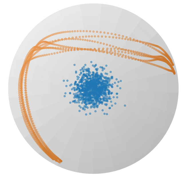
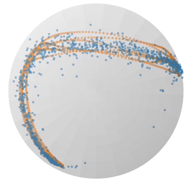
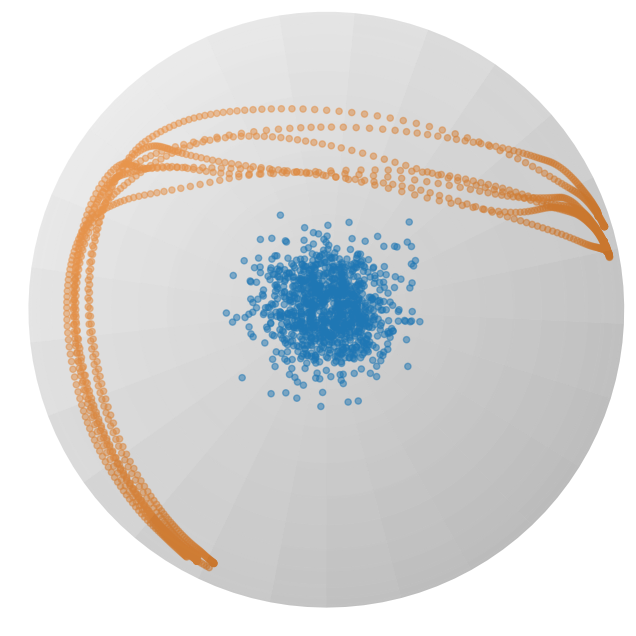
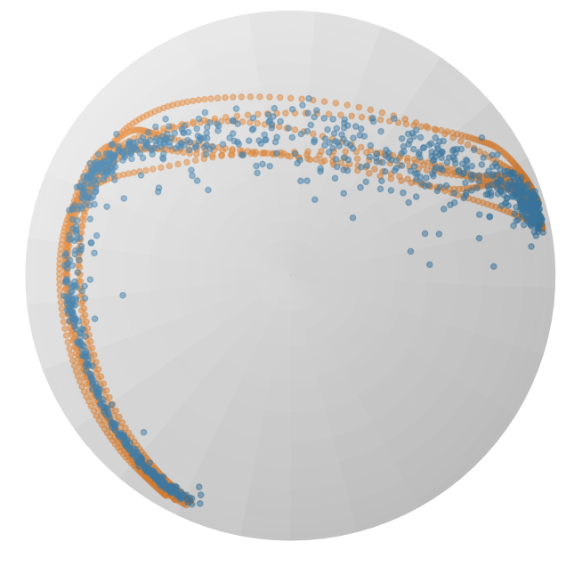
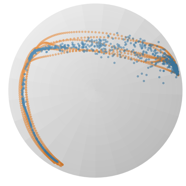
图 2:在球体流形上投影的 𝖫 形 LASA 数据集上训练的 RFM(顶部)和 SRFM(底部)的流动。橙色点表示训练数据集,而蓝色点显示在三个列的不同时间 t={0.0,1.0,1.5} 生成的概率路径。
IV-B2Stable Riemannian FMP
IV-B2 稳定黎曼流形匹配策略
初始参数 𝜽 ,先验和目标分布 p0 , p1 .
输出:学习到的向量场参数 𝜽 。
3 从均匀分布 𝒰[0,1] 中采样流时间步 t 。
4 样本噪声 𝒂0∼p0 .
5 联合采样动作序列 𝒂1∼p1 和相应的观测向量 𝒐 。
6 形成向量 𝝃1=[𝒂1,τ1] 和 𝝃0=[𝒂0,τ0] 。
7 通过 (14) 计算条件向量场 ut(𝝃t|𝝃1) 。
8 评估损失 ℓSRFMP ,如 (22) 中定义。
9 更新参数 𝜽 .
预定义的函数评估次数 N ,学习的向量场 v𝜽 ,观测向量 𝒐 和先验分布 p0 。
11 样本 𝒂0∼p0 ,并设置 t=0 , 𝝃0=[𝒂0,τ0] 。
13 更新时间步长 t=t+1 ,
18 在学习的黎曼向量场上的积分 𝝃t=Exp𝝃t−1(v𝜽(𝝃t−1,𝒐)Δt)
算法 2 SRFMP 训练和推理过程
Next, we introduce our extension, stable Riemannian flow matching (SRFM), which generalizes SFM [20] to Riemannian manifolds. Similarly as SFM, we define a time-invariant vector field u by augmenting the state space with the pseudo-time state τ, so that 𝝃=[𝒙,τ]. Notice that, in this case, 𝒙∈ℳ and thus 𝝃 lies on the product of Riemannian manifolds ℳ×ℝ. Importantly, Theorem 1 also holds for Riemannian autonomous systems, in which case ∇𝒙H(𝒙) denotes the Riemannian gradient of the positive scalar function H. We formulate H so that the pair (H,𝝃) satisfies (12) as,
接下来,我们介绍我们的扩展,稳定黎曼流匹配(SRFM),它将 SFM [20]推广到黎曼流形。与 SFM 类似,我们通过用伪时间状态 τ 扩展状态空间来定义时间不变向量场 u ,以便 𝝃=[𝒙,τ] 。请注意,在这种情况下, 𝒙∈ℳ ,因此 𝝃 位于黎曼流形 ℳ×ℝ 的乘积上。重要的是,定理 1 也适用于黎曼自治系统,在这种情况下, ∇𝒙H(𝒙) 表示正标量函数 H 的黎曼梯度。我们将 H 公式化,使得对 (H,𝝃) 满足(12),如下所示:
| H(𝝃|𝝃1)=12Log𝝃1(𝝃)⊤𝑨Log𝝃1(𝝃), | (18) |
which leads to the Riemannian vector field,
这导致了黎曼向量场,
| u(𝝃|𝝃1)=−∇𝝃H(𝝃)⊤=−𝑨Log𝝃1(𝝃). | (19) |
By setting the positive-definite matrix 𝑨 as in (15), we obtain the Riemannian vector field,
通过设置正定矩阵 𝑨 如(15)所示,我们得到黎曼向量场,
| u(𝝃t|𝝃1)=[u𝒙(𝒙t|𝒙1)uτ(τt|τ1)]=[−λ𝒙Log𝒙1(𝒙0)−λτ(τ0−τ1)], | (20) |
which generates the stable Riemannian flow,
生成稳定的黎曼流,
| ψt(𝝃0|𝝃1)=[ψt(𝒙0|𝒙1)ψt(τ0|τ1)]=[Exp𝒙1(e−λ𝒙tLog𝒙1(𝒙0))τ1+e−λτt(τ0−τ1)]. | (21) |
The parameters λ𝒙 and λτ have the same influence as in the Euclidean case. Notice that the spatial part of the stable flow (21) closely resembles the geodesic flow (8) proposed in [16]. Figure 2 shows an example of learned RFM and SRFM flows at times t={0,1,1.5}. The RFM flow diverges from the target distribution at times t>1, while the SRFM flow is stable and adheres to the target distribution for t≥1.
参数 λ𝒙 和 λτ 与欧几里得情况具有相同的影响。请注意,稳定流(21)的空间部分与[16]中提出的测地流(8)非常相似。图 2 显示了在时间 t={0,1,1.5} 处学习到的 RFM 和 SRFM 流的示例。RFM 流在时间 t>1 处偏离目标分布,而 SRFM 流在 t≥1 处稳定并遵循目标分布。
Finally, the process to induce this stable behavior into the RFMP flow involves two main changes: (1) We define an augmented action horizon vector 𝝃=[𝒂s,…,𝒂s+Tp,τ], and; (2) We regress the observation-conditioned Riemannian vector field v(𝝃|𝒐;𝜽) against the stable Riemannian vector field u(𝝃|𝝃1) defined in (19), where 𝒐 denotes the observation vector. The model is then trained to minimize the SRFMP loss,
最后,将这种稳定行为引入 RFMP 流的过程涉及两个主要变化:(1)我们定义了一个扩展的动作视界向量 𝝃=[𝒂s,…,𝒂s+Tp,τ] ,以及;(2)我们将观察条件的黎曼向量场 v(𝝃|𝒐;𝜽) 回归到(19)中定义的稳定黎曼向量场 u(𝝃|𝝃1) ,其中 𝒐 表示观察向量。然后训练模型以最小化 SRFMP 损失。
| ℓSRFMP=𝔼t,q(𝒂1),p(𝒂0)∥v(𝝃t|𝒐;𝜽)−u(𝝃t|𝝃1)∥g𝒂t2. | (22) |
This approach, hereinafter referred to as stable Riemannian flow matching policy (SRFMP), is summarized in Algorithm 2. The learned SRFMP vector field drives the flow to converge to the target distribution within a certain time horizon, ensuring that it remains within this distribution, as illustrated by the bottom row of Figures 1 and 2. In contrast, the RFMP vector field may drift the flow away from the target distribution at t>1 (see Figures 1 and 2, top row). Therefore, SRFMPs provide flexibility and increased robustness in designing the generation process, while RFMPs are more sensitive to the integration process.
这种方法(以下简称稳定黎曼流匹配策略 (SRFMP))在算法 2 中进行了总结。学习到的 SRFMP 向量场驱动流在一定时间范围内收敛到目标分布,确保其保持在该分布内,如图 1 和图 2 的底行所示。相比之下,RFMP 向量场可能会在 t>1 处将流漂移离目标分布(见图 1 和图 2 的顶行)。因此,SRFMP 在设计生成过程时提供了灵活性和更高的鲁棒性,而 RFMP 对积分过程更为敏感。
IV-B3Solving the SRFMP ODE
IV-B3 求解 SRFMP ODE
As previously discussed, querying SRFMP policies involves integrating the learned vector field along the time interval t=[0,T] with time boundary T. To do so, we use the projected Euler method, which integrates the vector field on the tangent space for one Euler step and then projects the resulting vector onto the manifold ℳ. Assuming an Euclidean setting and that v(𝝃|𝒐;𝜽) is perfectly learned, this corresponds to recursively applying,
如前所述,查询 SRFMP 策略涉及在时间间隔 t=[0,T] 内沿着时间边界 T 积分学习的向量场。为此,我们使用投影欧拉方法,该方法在切空间上对向量场进行一次欧拉步积分,然后将所得向量投影到流形 ℳ 上。假设欧几里得设置和 v(𝝃|𝒐;𝜽) 完全学习,这相当于递归应用,
| 𝒙t+1=𝒙t+v𝒙(𝒙t|𝒐;𝜽)Δt≈𝒙t+λ𝒙(𝒙1−𝒙t)Δt, | (23) |
with time step Δt and v𝒙 following the same partitioning as u𝒙 in (20). The time step Δt is typically set as Δt=T/N, where N is the total number of ODE steps. Here we propose to leverage the structure of SRFMP to choose the time step Δt in order to further speed up the inference time of RFMP. Specifically, we observe that the recursion (23) leads to,
时间步长 Δt 和 v𝒙 遵循 (20) 中的 u𝒙 相同的划分。时间步长 Δt 通常设置为 Δt=T/N ,其中 N 是 ODE 步骤的总数。这里我们提出利用 SRFMP 的结构来选择时间步长 Δt ,以进一步加快 RFMP 的推理时间。具体来说,我们观察到递归 (23) 导致,
| 𝒙t=(1−λ𝒙Δt)n(𝒙0−𝒙1)+𝒙1, | (24) |
after n time steps. It is easy to see that 𝒙t converges to 𝒙1 after a single time step when setting Δt=1/λ𝒙.
在 n 个时间步之后。很容易看出,当设置 Δt=1/λ𝒙 时, 𝒙t 在一个时间步之后收敛到 𝒙1 。
In the Riemannian case, assuming that v(𝝃|𝒐;𝜽) approximately equals the Riemannian vector field (20), we obtain,
在黎曼情况下,假设 v(𝝃|𝒐;𝜽) 大致等于黎曼向量场(20),我们得到,
| 𝒙t+1=Exp𝒙t(v𝒙(𝒙|𝒐;𝜽)Δt)≈Exp𝒙t(λ𝒙Log𝒙t(𝒙1)Δt). | (25) |
Similarly, it is easy to see that the Riemannian flow converges to 𝒙1 after a single time step for Δt=1/λ𝒙. Importantly, this strategy assumes that the learned vector field is perfectly learned and thus equals the target vector field. However, this is often not the case in practice. However, our experiments show that the flow obtained solving the SRFMP ODE with a single time step Δt=1/λ𝒙 generally leads to the target distribution. In practice, we set Δt to 1/λ𝒙 for the first time step, and to a smaller value afterwards for refining the flow.
同样,很容易看出黎曼流在单个时间步后收敛到 𝒙1 对于 Δt=1/λ𝒙 。重要的是,这种策略假设学习到的向量场是完美学习的,因此等于目标向量场。然而,这在实践中往往不是这种情况。然而,我们的实验表明,通过单个时间步 Δt=1/λ𝒙 求解 SRFMP ODE 获得的流通常会导致目标分布。在实践中,我们将 Δt 设置为 1/λ𝒙 用于第一个时间步,然后设置为较小的值以优化流。
VExperiments V 实验
We thoroughly evaluate the performance of RFMP and SRFMP on a set of six simulation settings and two real-world tasks. The simulated benchmarks are: (1) The Push-T task from [2]; (2) A Sphere Push-T task, which we introduce as a Riemannian benchmark; and (3)-(6) Four tasks (Lift, Can, Square, and Tool Hang) from the large-scale robot manipulation benchmark Robomimic [10]. The real-world robot tasks correspond to: (1) A Pick & Place task; and (2) A Mug Flipping task. Collectively, these eight tasks serve as a benchmark to evaluate (1) the performance, (2) the training time, and (3) the inference time of RFMP and SRFMP with respect to state-of-the-art generative policies, i.e., DP and extensions thereof.
我们在六个模拟设置和两个现实世界任务中全面评估了 RFMP 和 SRFMP 的性能。模拟基准是:(1) Push-T 任务 [2];(2) 我们引入的球体 Push-T 任务,作为黎曼基准;(3)-(6) 来自大规模机器人操作基准 Robomimic [10]的四个任务(Lift、Can、Square 和 Tool Hang)。现实世界的机器人任务对应于:(1) 拾取和放置任务;(2) 翻转杯子任务。这八个任务共同作为基准来评估 RFMP 和 SRFMP 相对于最先进生成策略(即 DP 及其扩展)的(1) 性能、(2) 训练时间和(3) 推理时间。
V-AImplementation Details
V-A 实施细节
To establish a consistent experimental framework, we first introduce the neural network architectures employed in RFMP and SRFMP across all tasks. We then describe the considered baselines, and our overall evaluation methodology.
为了建立一致的实验框架,我们首先介绍在所有任务中使用的 RFMP 和 SRFMP 的神经网络架构。然后,我们描述所考虑的基线,以及我们的整体评估方法。
V-A1RFMP and SRFMP Implementation
V-A1 RFMP 和 SRFMP 实现
Our RFMP implementation builds on the RFM framework from Chen and Lipman [16]. We parameterized the vector field vt(𝒂|𝒐;𝜽) using the UNet architecture employed in DP [2], which consists of 3 layers with downsampling dimensions of (256,512,1024) and (128,256,512) for simulated and real-world tasks. Each layer employs a 1-dimensional convolutional residual network as proposed in [29]. We implement a Feature-wise Linear Modulation (FiLM) [58] to incorporate the observation condition vector 𝒐 and time step t into the UNet. Instead of directly feeding the FM time step t as a conditional variable, we first project it into a higher-dimensional space using a sinusoidal embedding module, similarly to DP. For tasks with image-based observations, we leverage the same vision perception backbone as in DP [2]. Namely, we use a standard ResNet-18 in which we replace: (1) the global average pooling with a spatial softmax pooling, and (2) BatchNorm with GroupNorm. Our SRFMP implementation builds on the SFM framework [20]. We implement the same UNet as RFMP to represent v𝒙 by replacing the time step t by the temperature parameter τ. We introduce an additional Multi-Layer Perceptron (MLP) to learn vτ. As for t in RFMP, we employed a sinusoidal embedding for the input τ. The boundaries τ0 and τ1 are set to 0 and 1 in all experiments.
我们的 RFMP 实现基于 Chen 和 Lipman [16] 的 RFM 框架。我们使用 DP [2] 中采用的 UNet 架构对向量场 vt(𝒂|𝒐;𝜽) 进行了参数化,该架构由 3 层组成,具有 (256,512,1024) 和 (128,256,512) 的下采样维度,用于模拟和现实任务。每一层都采用了 [29] 中提出的 1 维卷积残差网络。我们实现了特征线性调制 (FiLM) [58],将观测条件向量 𝒐 和时间步长 t 融入 UNet。我们没有直接将 FM 时间步长 t 作为条件变量,而是首先使用正弦嵌入模块将其投射到更高维空间,类似于 DP。对于基于图像的观测任务,我们利用与 DP [2] 中相同的视觉感知骨干网络。即,我们使用标准的 ResNet- 18 ,其中我们替换了:(1) 全局平均池化为空间 softmax 池化,(2) BatchNorm 为 GroupNorm。我们的 SRFMP 实现基于 SFM 框架 [20]。我们实现了与 RFMP 相同的 UNet,通过将时间步长 t 替换为温度参数 τ 来表示 v𝒙 。 我们引入了一个额外的多层感知器(MLP)来学习 vτ 。至于 RFMP 中的 t ,我们为输入 τ 采用了正弦嵌入。所有实验中的边界 τ0 和 τ1 设置为 0 和 1 。
We implement different prior distributions for different tasks. For the Euclidean Push-T and the four Robomimic tasks, the action space is ℝd and we thus define the prior distribution as a Euclidean Gaussian distribution for both RFMP and SRFMP. For the Sphere Push-T, the action space is the hypersphere 𝒮2. In this case, we test two types of Riemannian prior distribution, namely a spherical uniform distribution, and a wrapped Gaussian distribution [59, 60], illustrated in Figure 3. Regarding the real robot tasks, the task space is defined as the product manifold ℳ=ℝ3×𝒮3×ℝ1, whose components represent the position, orientation (encoded as quaternions), and opening of the gripper. The Euclidean and hypersphere parts employ Euclidean Gaussian distributions and a wrapped Gaussian distribution, respectively.
我们为不同的任务实现了不同的先验分布。对于 Euclidean Push-T 和四个 Robomimic 任务,动作空间是 ℝd ,因此我们将先验分布定义为 RFMP 和 SRFMP 的欧几里得高斯分布。对于 Sphere Push-T,动作空间是超球面 𝒮2 。在这种情况下,我们测试了两种类型的黎曼先验分布,即球面均匀分布和缠绕高斯分布[59, 60],如图 3 所示。关于真实机器人任务,任务空间定义为乘积流形 ℳ=ℝ3×𝒮3×ℝ1 ,其组件表示位置、方向(编码为四元数)和夹爪的开合。欧几里得部分和超球面部分分别采用欧几里得高斯分布和缠绕高斯分布。
表 I:所有实验的超参数:原始和裁剪图像的分辨率,使用 RFMP 和 SRFMP 学习的向量场参数数量,ResNet 参数数量,训练周期和批量大小。
| Experiment 实验 | Image res. 图像分辨率。 | Crop res. 作物资源。 | RFMP VF Num. params RFMP VF 参数数量 | SRFMP VF Num. params | ResNet params ResNet 参数 | Epochs 时期 | Batch size 批量大小 |
|---|---|---|---|---|---|---|---|
| Push-T Tasks 推-T 任务 | |||||||
| Eucl. Push-T task 欧几里得推-T 任务 | 96×96 | 84×84 | 8.0×1007 | 8.14×1007 | 1.12×1007 | 300 | 256 |
| Sphere Push-T task 球体推-T 任务 | 100×100 | 84×84 | 8.0×1007 | 8.14×1007 | 1.12×1007 | 300 | 256 |
| State-based Robomimic 基于状态的 Robomimic | |||||||
| Lift 提升 | N.A. | N.A. | 6.58×1007 | 6.68×1007 | N.A. | 50 | 256 |
| Can 能 | N.A. | N.A. | 6.58×1007 | 6.68×1007 | N.A. | 50 | 256 |
| Square 正方形 | N.A. | N.A. | 6.58×1007 | 6.68×1007 | N.A. | 50 | 512 |
| Tool Hang 工具挂起 | N.A. | N.A. | 6.58×1007 | 6.68×1007 | N.A. | 100 | 512 |
| Vision-based Robomimic 基于视觉的 Robomimic | |||||||
| Lift 提升 | 2×84×84 | 2×76×76 | 9.48×1007 | 9.69×1007 | 2×1.12×1007 | 100 | 256 |
| Can 能 | 2×84×84 | 2×76×76 | 9.48×1007 | 9.69×1007 | 2×1.12×1007 | 100 | 256 |
| Square 正方形 | 2×84×84 | 2×76×76 | 9.48×1007 | 9.69×1007 | 2×1.12×1007 | 100 | 512 |
| Real-world experiments 现实世界实验 | |||||||
| Pick & place 拣选与放置 | 320×240 | 288×216 | 2.51×1007 | 2.66×1007 | 1.12×1007 | 300 | 256 |
| Rotate mug 旋转杯子 | 320×240 | 256×192 | 2.51×1007 | 2.66×1007 | 1.12×1007 | 300 | 256 |
For all experiments, we optimize the network parameters of RFMP and SRFMP using AdamW [61] with a learning rate of η=1×10⁻⁴ and weight decay of wd=0.001 based on an exponential moving averaging (EMA) framework on the weights [62] with a decay of wEMA=0.999. Moreover, we use an action prediction horizon Tp=16, an action horizon Ta=Tp/2, and an observation horizon To=2. We set the SRFMP parameters as λ𝒙=λτ=2.5. Table I summarizes the image resolution, number of parameters, and number of training epochs used in each experiment.
对于所有实验,我们使用 AdamW [61] 优化 RFMP 和 SRFMP 的网络参数,学习率为 η=1×10⁻⁴ ,权重衰减为 wd=0.001 ,基于权重的指数移动平均 (EMA) 框架 [62],衰减为 wEMA=0.999 。此外,我们使用动作预测视界 Tp=16 ,动作视界 Ta=Tp/2 和观察视界 To=2 。我们将 SRFMP 参数设置为 λ𝒙=λτ=2.5 。表格总结了每个实验中使用的图像分辨率、参数数量和训练周期数。
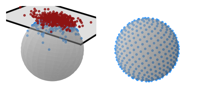
图 3:Sphere Push-T 任务中使用的先验分布的二维可视化:包裹高斯分布(左)和球面均匀分布(右)。球面高斯分布是通过首先从球面切空间上的欧几里得高斯分布中采样(红点),然后通过指数映射将样本投影到球面流形 𝒮d (蓝点)上获得的。球面均匀分布是通过对零均值欧几里得高斯分布的样本进行归一化计算得出的。
V-A2Baselines V-A2 基线
In the original DP paper [2], the policy is trained using either Denoising Diffusion Probabilistic Model (DDPM) [12] or Denoising Diffusion Implicit Model (DDIM) [13]. In this paper, we prioritize faster inference and thus employ DDIM-based DP for all our experiments. We train DDIM with 100 denoising steps. The prior distribution is a standard Gaussian distribution unless explicitly mentioned. During training we use the same noise scheduler as in [2], the optimizer AdamW with the same learning rate and weight decay as for RFMP and SRFMP. Note that DP does not handle data on Riemannian manifolds, and thus does not guarantee that the resulting trajectories lie on the manifold of interest for tasks with Riemannian action spaces, e.g., the Sphere Push-T and real-world robot experiments. In these cases, we post-process the trajectories obtained during inference and project them on the manifold. In the case of the hypersphere manifold, the projection corresponds to a unit-norm normalization. We also compare RFMP and SRFMP against CP [3] on the Robomimic tasks with vision-based observations. To do so, we use the performance values reported in [3].
在原始的 DP 论文 [2] 中,策略使用去噪扩散概率模型 (DDPM) [12] 或去噪扩散隐式模型 (DDIM) [13] 进行训练。在本文中,我们优先考虑更快的推理,因此在所有实验中都采用基于 DDIM 的 DP。我们使用 100 个去噪步骤训练 DDIM。先验分布是标准高斯分布,除非明确说明。在训练期间,我们使用与 [2] 中相同的噪声调度器,优化器 AdamW 具有与 RFMP 和 SRFMP 相同的学习率和权重衰减。请注意,DP 不处理黎曼流形上的数据,因此不能保证生成的轨迹位于具有黎曼动作空间的任务的感兴趣流形上,例如 Sphere Push-T 和现实世界的机器人实验。在这些情况下,我们对推理过程中获得的轨迹进行后处理,并将其投影到流形上。在超球面流形的情况下,投影对应于单位范数归一化。我们还将 RFMP 和 SRFMP 与 Robomimic 任务中基于视觉的观察的 CP [3] 进行比较。为此,我们使用 [3] 中报告的性能值。
V-A3Evaluation methodology
V-A3 评估方法
We evaluate RFMP, SRFMP, and DP using three key metrics: (1) The performance, computed as the average task-depending score across all trials, with 50 trials for each simulated task, and 10 trials for each real-world task; (2) The number of training epochs; and (3) The inference time. To provide a consistent measure of inference time across RFMP, SRFMP, and DP, we report it in terms of the number of function evaluations (NFE), which is proportional to the inference process time. Given that each function evaluation takes approximately the same time across all methods, inference time comparisons can be made directly based on NFE. For example, in real-world tasks, with an NFE of 2, DP requires around 0.0075s, while RFMP and SRFMP take approximately 0.0108s and 0.0113s, respectively. When NFE is increased to 5, DP takes around 0.0175s, while RFMP and SRFMP require about 0.021s and 0.0212s.
我们使用三个关键指标评估 RFMP、SRFMP 和 DP:(1)性能,计算为所有试验的平均任务依赖得分,每个模拟任务有 50 次试验,每个实际任务有 10 次试验;(2)训练周期数;(3)推理时间。为了在 RFMP、SRFMP 和 DP 之间提供一致的推理时间度量,我们以函数评估次数(NFE)来报告它,这与推理过程时间成正比。鉴于每次函数评估在所有方法中大致需要相同的时间,可以直接基于 NFE 进行推理时间比较。例如,在实际任务中,NFE 为 2 时,DP 需要大约 0.0075s ,而 RFMP 和 SRFMP 分别需要大约 0.0108s 和 0.0113s 。当 NFE 增加到 5 时,DP 需要大约 0.0175s ,而 RFMP 和 SRFMP 分别需要大约 0.021s 和 0.0212s 。
V-BPush-T Tasks
We first consider two simple Push-T tasks, namely the Euclidean Push-T proposed in [2], which was adapted from the Block Pushing task [8], and the Sphere Push-T task, which we introduce shortly. The goal of the Euclidean Push-T task, illustrated in Figure 4, is to push a gray T-shaped object to the designated green target area with a blue circular agent. The agent’s movement is constrained by a light gray square boundary. Each observation 𝒐 is composed of the 96×96 RGB image of the current scene and the agent’s state information. We introduce the Sphere Push-T task, visualized in Figure 4, to evaluate the performance of our models on the sphere manifold. Its environment is obtained by projecting the Euclidean Push-T environment on one half of a 2-dimensional sphere 𝒮2 of radius of 1. This is achieved by projecting the environment, normalized to a range [−1.5,1.5], from the plane z=1 to the sphere via a stereographic projection. The target area, the T-shaped object, and the agent then lie and evolve on the sphere. As in the Euclidean case, each observation 𝒐 is composed of the 96×96 RGB image of the current scene and the agent’s state information on the manifold. All models (i.e., RFMP, SRFMP, DP) are trained for 300 epochs in both settings. During testing, we choose the best validation epoch and only roll out 500 steps in the environment with an early stop rule terminating the execution when the coverage area is over 95% of the green target area. The score for both Euclidean and Sphere Push-T tasks is the maximum coverage ratio during execution. The tests are performed with 50 different initial states not present in the training set.
我们首先考虑两个简单的 Push-T 任务,即[2]中提出的欧几里得 Push-T 任务,该任务改编自 Block Pushing 任务[8],以及我们即将介绍的 Sphere Push-T 任务。欧几里得 Push-T 任务的目标如图 4 所示,是用蓝色圆形代理将灰色 T 形物体推到指定的绿色目标区域。代理的移动受到浅灰色方形边界的限制。每个观测 𝒐 由当前场景的 96×96 RGB 图像和代理的状态信息组成。我们引入了 Sphere Push-T 任务,如图 4 所示,以评估我们模型在球面流形上的性能。其环境是通过将欧几里得 Push-T 环境投影到半径为 1 的 2 维球体的一个半球上获得的。这是通过将归一化到范围 [−1.5,1.5] 的环境从平面 z=1 通过立体投影投影到球体上来实现的。目标区域、T 形物体和代理然后在球体上存在和演变。与欧几里得情况一样,每个观测 𝒐 由当前场景的 96×96 RGB 图像和流形上的代理状态信息组成。 所有模型(即 RFMP、SRFMP、DP)在两种设置下均训练 300 个周期。在测试期间,我们选择最佳验证周期,并且在环境中仅执行 500 步,当覆盖区域超过绿色目标区域的 95% 时,提前停止执行。欧几里得和球面推送-T 任务的得分是执行期间的最大覆盖率。测试在训练集中不存在的 50 个不同初始状态下进行。
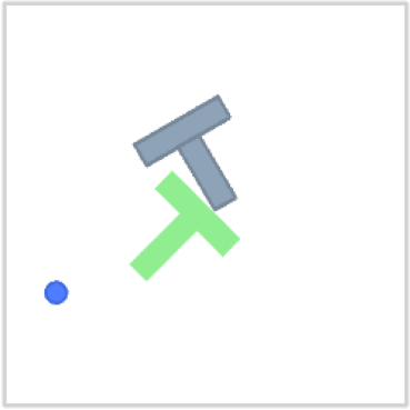
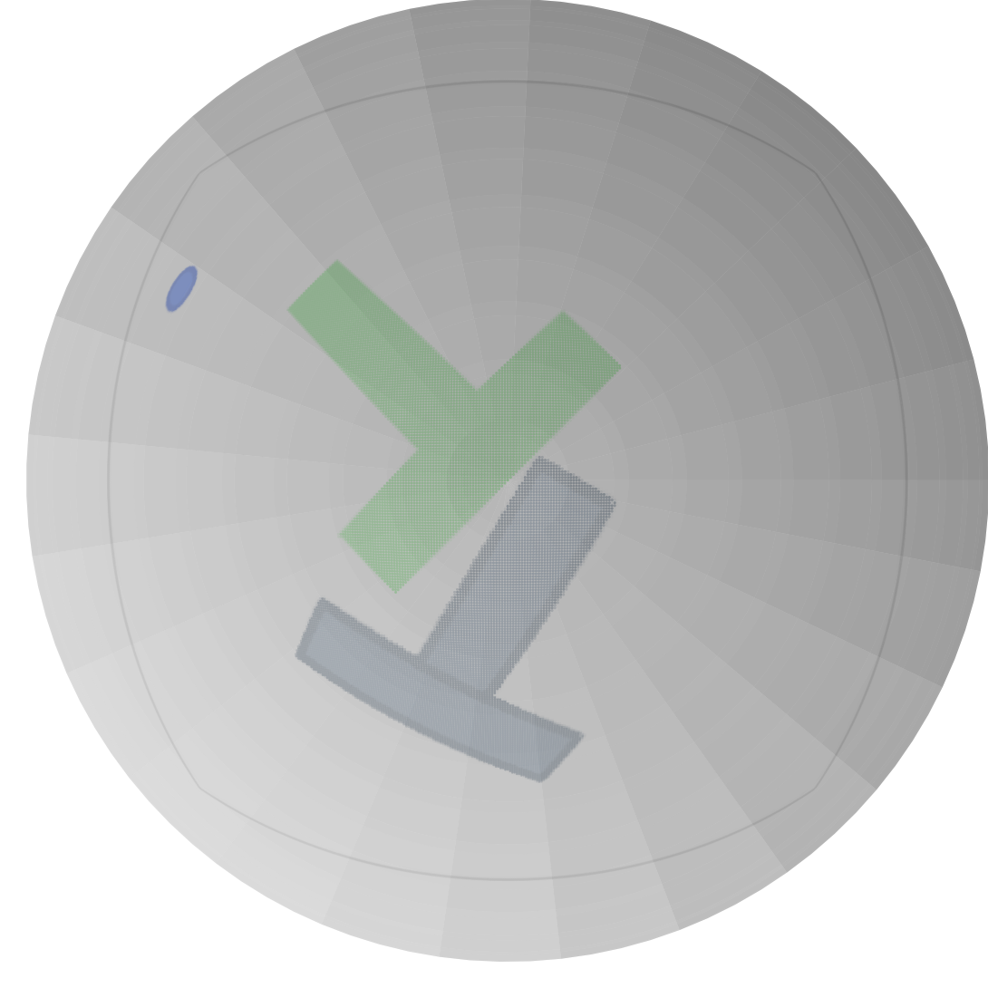
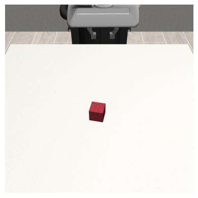
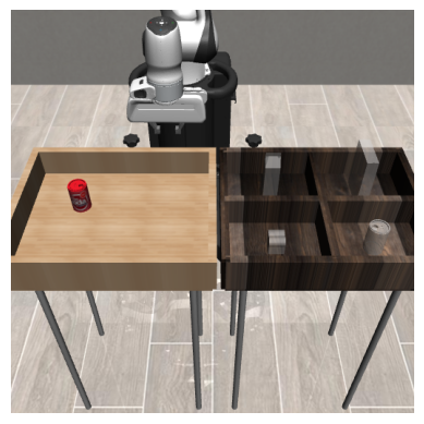
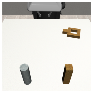
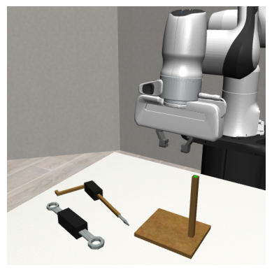
图 4:仿真基准:Euclidean Push-T [2],Sphere Push-T,以及来自 Robomimic [10]的四个任务:Lift,Can,Square,Tool Hang。
V-B1Euclidean Push-T V-B1 欧几里得推-T
First, we evaluate the performance of RFMP and SRFMP in the Euclidean case for different number of function evaluations in the testing phase. The models are trained with the default parameters described in Section V-A1. Table II shows the success rate of RFMP and SRFMP for different NFEs. We observe that both RFMP and SRFMP achieve similar success rates overall. While SRFMP demonstrates superior performance with a single NFE, RFMP achieves higher success rates with more NFEs. We hypothesize that this behavior arises from the fact that, due to the equality λ𝒙=λτ, the SRFMP conditional probability path resembles the optimal transport map between the prior and target distributions as in [15]. This, along with the stability framework of SRFMP, allows us to automatically choose the timestep during inference via (24), which enhances convergence in a single step. When comparing our approaches with DP, we observe that DP performs drastically worse than both RFMP and SRFMP for a single NFE, achieving a score of only 10.9%. Nevertheless, the performance of DP improves when increasing the NFE and matches that of our approaches for 10 NFE.
首先,我们在欧几里得情况下评估 RFMP 和 SRFMP 在测试阶段不同函数评估次数下的性能。模型使用 V-A1 节中描述的默认参数进行训练。表 II 显示了 RFMP 和 SRFMP 在不同 NFE 下的成功率。我们观察到,RFMP 和 SRFMP 总体上都达到了相似的成功率。虽然 SRFMP 在单次 NFE 中表现出色,但 RFMP 在更多 NFE 下达到了更高的成功率。我们假设这种行为是由于等式 λ𝒙=λτ ,SRFMP 条件概率路径类似于[15]中的先验和目标分布之间的最优传输映射。这与 SRFMP 的稳定性框架一起,使我们能够通过(24)在推理过程中自动选择时间步长,从而在一步中增强收敛性。与 DP 相比,我们观察到 DP 在单次 NFE 中表现远不如 RFMP 和 SRFMP,仅获得 10.9% 的分数。然而,随着 NFE 的增加,DP 的性能有所提高,并在 10 NFE 时与我们的方法相匹配。
表 II:欧几里得 Push-T:NFE 对策略的影响
| NFE | ||||
|---|---|---|---|---|
| Policy 政策 | 1 | 3 | 5 | 10 |
| RFMP | 0.848 | 0.855 | 0.923 | 0.891 |
| SRFMP | 0.875 | 0.851 | 0.837 | 0.856 |
| DP | 0.109 | 0.79 | 0.838 | 0.862 |
Next, we ablate the action prediction horizon Tp, observation horizon To, learning rate η, and weight decay wd for RFMP and SRFMP. We consider 3 different values for each, while setting the other hyperparameters to their default values, and test the resulting models with 5 different NFE. For SRFMP, we additionally ablate the parameters λ𝒙 and λτ for 3 different ratios λ𝒙/λτ and 4 values for each ratio. Each setup is tested with 50 seeds, resulting in a total of 2250 and 4000 experiments for RFMP and SRFMP. The results are reported in Tables III and IV, respectively. We observe that a short observation horizon To=2 leads to the best performance for both models. This is consistent with the task, as the current and previous images accurately provide the required information for the next pushing action, while the actions associated with past images rapidly become outdated. Moreover, we observe that an action prediction horizon Tp=16 leads to the highest score. We hypothesize that this horizon allows the model to maintain temporal consistency, while providing frequent enough updates of the actions according to the current observations. Concerning SRFMP, we find that λ𝒙=λτ=2.5 leads to the highest success rates. Interestingly, this choice leads to the ratio λ𝒙/λτ=1, in which case the flow of 𝒙 follows the Gaussian CFM (6) of [15] with σ→0 for τ=[0,1], see [20, Cor 4.12]. In the next experiments, we use the default parameters resulting from our ablations, i.e., Tp=16, To=2, η=1×10⁻⁴, wd=0.001, and λ𝒙=λτ=2.5.
接下来,我们对 RFMP 和 SRFMP 的动作预测视野 Tp 、观察视野 To 、学习率 η 和权重衰减 wd 进行消融。我们考虑了每个参数的 3 个不同值,同时将其他超参数设置为默认值,并使用 5 个不同的 NFE 测试生成的模型。对于 SRFMP,我们还对参数 λ𝒙 和 λτ 进行了消融,考虑了 3 个不同的比率,每个比率有 λ𝒙/λτ 和 4 个值。每个设置使用 50 个种子进行测试,最终对 RFMP 和 SRFMP 进行了 2250 和 4000 次实验。结果分别在表 III 和表 IV 中报告。我们观察到,短观察视野 To=2 对两种模型的性能最佳。这与任务一致,因为当前和以前的图像准确地提供了下一次推送动作所需的信息,而与过去图像相关的动作很快就会过时。此外,我们观察到,动作预测视野 Tp=16 导致了最高分。我们假设这个视野允许模型保持时间一致性,同时根据当前观察结果提供足够频繁的动作更新。 关于 SRFMP,我们发现 λ𝒙=λτ=2.5 导致了最高的成功率。有趣的是,这一选择导致了 λ𝒙/λτ=1 的比率,在这种情况下, 𝒙 的流动遵循[15]的高斯 CFM(6),其中 σ→0 对于 τ=[0,1] ,见[20,Cor 4.12]。在接下来的实验中,我们使用从消融实验中得出的默认参数,即 Tp=16 , To=2 , η=1×10⁻⁴ , wd=0.001 和 λ𝒙=λτ=2.5 。
表 III:RFMP 超参数消融在欧几里得 Push-T 上的表现
| Parameter 参数 | Values 值 | Success rate 成功率 | ||||
|---|---|---|---|---|---|---|
| NFE | 1 | 3 | 5 | 10 | 100 | |
| To | 𝟐 | 0.848 | 0.855 | 0.923 | 0.891 | 0.91 |
| 8 | 0.195 | 0.16 | 0.154 | 0.168 | 0.179 | |
| 16 | 0.135 | 0.143 | 0.14 | 0.133 | 0.135 | |
| 8 | 0.754 | 0.835 | 0.827 | 0.839 | 0.85 | |
| 𝟏𝟔 | 0.848 | 0.855 | 0.923 | 0.891 | 0.91 | |
| Tp | 32 | 0.799 | 0.906 | 0.878 | 0.929 | 0.93 |
| η | 𝟏×𝟏𝟎−𝟒 | 0.848 | 0.855 | 0.923 | 0.891 | 0.91 |
| 5×10⁻⁵ | 0.797 | 0.863 | 0.843 | 0.897 | 0.889 | |
| 1×10⁻⁵ | 0.641 | 0.771 | 0.805 | 0.88 | 0.841 | |
| 0.001 | 0.848 | 0.855 | 0.923 | 0.891 | 0.91 | |
| 0.005 | 0.846 | 0.882 | 0.875 | 0.866 | 0.856 | |
| wd | 0.01 | 0.868 | 0.831 | 0.842 | 0.927 | 0.853 |
表 IV:SRFMP 超参数消融在欧几里得 Push-T 上的表现
| Parameter 参数 | Values 值 | Success rate 成功率 | |||
|---|---|---|---|---|---|
| NFE | 1 | 3 | 5 | 10 | |
| To | 𝟐 | 0.875 | 0.851 | 0.837 | 0.856 |
| 8 | 0.124 | 0.139 | 0.147 | 0.13 | |
| 16 | 0.145 | 0.138 | 0.149 | 0.144 | |
| 8 | 0.816 | 0.726 | 0.592 | 0.318 | |
| 𝟏𝟔 | 0.875 | 0.851 | 0.837 | 0.856 | |
| Tp | 32 | 0.852 | 0.861 | 0.881 | 0.829 |
| η | 1.0×𝟏𝟎−𝟒 | 0.875 | 0.851 | 0.837 | 0.856 |
| 5×10⁻⁵ | 0.754 | 0.621 | 0.456 | 0.334 | |
| 1×10⁻⁵ | 0.602 | 0.56 | 0.443 | 0.288 | |
| 0.001 | 0.875 | 0.851 | 0.837 | 0.856 | |
| 0.005 | 0.837 | 0.826 | 0.826 | 0.684 | |
| wd | 0.01 | 0.733 | 0.75 | 0.768 | 0.571 |
| λ𝒙λτ | 1 0.2 | 0.74 | 0.614 | 0.494 | 0.457 |
| 1 1 | 0.85 | 0.777 | 0.608 | 0.416 | |
| 1 6 | 0.87 | 0.768 | 0.753 | 0.812 | |
| 2.5 0.2 | 0.832 | 0.392 | 0.576 | 0.549 | |
| 2.5 2.5 | 0.875 | 0.851 | 0.837 | 0.856 | |
| 2.5 15 | 0.832 | 0.799 | 0.789 | 0.807 | |
| 5 1 | 0.796 | 0.741 | 0.614 | 0.513 | |
| 5 5 | 0.845 | 0.825 | 0.797 | 0.642 | |
| 5 30 | 0.822 | 0.830 | 0.772 | 0.743 | |
| 7.5 1.5 | 0.799 | 0.685 | 0.442 | 0.456 | |
| 7.5 7.5 | 0.787 | 0.8 | 0.809 | 0.633 | |
| 7.5 45 | 0.782 | 0.817 | 0.844 | 0.814 | |
V-B2Sphere Push-T
Next, we test the ability of RFMP and SRFMP to generate motions on non-Euclidean manifolds with the Sphere Push-T task. We evaluate two types of Riemannian prior distributions for RFMP and SRFMP, namely a spherical uniform distribution and wrapped Gaussian distribution. We additionally consider a Euclidean Gaussian distribution for DP. Notice that the actions generated by DP are normalized in a post-processing step to ensure that they belong to the sphere. The corresponding performance are reported in Table V. Our results indicate that the choice of prior distribution significantly impacts the performance of both RFMP and SRFMP. Specifically, we observe that RFMP and SRFMP with a uniform sphere distribution consistently outperform their counterparts with wrapped Gaussian distribution. We hypothesize that RFMP or SRFMP benefit from having samples that are close to the data support, which leads to simpler vector fields to learn. In other words, uniform distribution provides more samples around the data distribution, which potentially lead to simpler vector fields. DP exhibit poor performance with sphere-based prior distributions, suggesting its ineffectiveness in handling such priors. Instead, DP’s performance drastically improves when using a Euclidean Gaussian distribution and higher NFE. Note that this high performance does not scale to higher dimensional settings as already evident in the real-world experiments reported in Section V-D, where the effect of ignoring the geometry of the parameters exacerbates, which is a known issue when naively operating with Riemannian data [63]. Importantly, SRFMP is consistently more robust to NFE and achieves high performance with a single NFE, leading to shorter inference times for similar performance compared to RFMP and DP.
接下来,我们测试了 RFMP 和 SRFMP 在非欧几里得流形上生成运动的能力,使用了 Sphere Push-T 任务。我们评估了两种用于 RFMP 和 SRFMP 的黎曼先验分布,即球面均匀分布和包裹高斯分布。我们还考虑了用于 DP 的欧几里得高斯分布。请注意,DP 生成的动作在后处理步骤中被归一化,以确保它们属于球面。相应的性能报告在表 V 中。我们的结果表明,先验分布的选择显著影响了 RFMP 和 SRFMP 的性能。具体来说,我们观察到,具有均匀球面分布的 RFMP 和 SRFMP 始终优于其具有包裹高斯分布的对应物。我们假设 RFMP 或 SRFMP 受益于接近数据支持的样本,这导致了更简单的向量场学习。换句话说,均匀分布在数据分布周围提供了更多的样本,这可能导致更简单的向量场。DP 在基于球面的先验分布下表现不佳,表明其在处理此类先验分布时效果不佳。 相反,当使用欧几里得高斯分布和更高的 NFE 时,DP 的性能显著提高。请注意,这种高性能并不能扩展到更高维度的设置中,这在第 V-D 节报告的实际实验中已经很明显,在这些实验中,忽略参数几何的影响加剧了这一问题,这是在处理黎曼数据时天真操作时的已知问题[63]。重要的是,SRFMP 对 NFE 始终更具鲁棒性,并且在单个 NFE 下实现高性能,从而在与 RFMP 和 DP 相似的性能下缩短推理时间。
表 V:先验分布对球推-T 任务的影响
| NFE | ||||
|---|---|---|---|---|
| Policy 政策 | 1 | 3 | 5 | 10 |
| RFMP sphere uniform RFMP 球体均匀 | 0.871 | 0.746 | 0.77 | 0.817 |
| RFMP sphere Gaussian RFMP 球面高斯 | 0.587 | 0.724 | 0.748 | 0.733 |
| SRFMP sphere uniform | 0.772 | 0.736 | 0.796 | 0.829 |
| SRFMP sphere Gaussian SRFMP 球面高斯 | 0.707 | 0.706 | 0.735 | 0.707 |
| DP sphere uniform DP 球均匀 | 0.274 | 0.261 | 0.235 | 0.197 |
| DP sphere Gaussian DP 球高斯 | 0.170 | 0.162 | 0.231 | 0.227 |
| DP euclidean Gaussian DP 欧几里得高斯 | 0.227 | 0.796 | 0.813 | 0.885 |
表 VI:积分时间对 RFMP 和 SRFMP 的影响
| Euclidean Push-T 欧几里得推-T | t=1.0 | t=1.2 | t=1.6 |
|---|---|---|---|
| RFMP | 0.855 | 0.492 | 0.191 |
| SRFMP | 0.862 | 0.851 | 0.829 |
| Sphere Push-T 球体推-T | t=1.0 | t=1.2 | t=1.6 |
| RFMP | 0.736 | 0.574 | 0.264 |
| SRFMP | 0.727 | 0.736 | 0.685 |
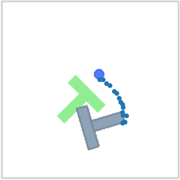
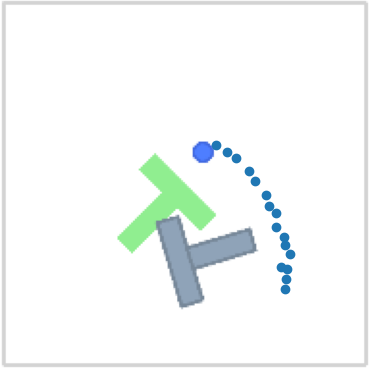

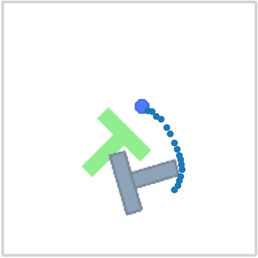


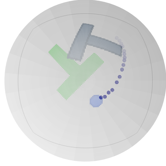

图 5:由 RFMP(第一和第三行)和 SRFMP(第二和第四行)在 Push-T 任务上训练生成的动作序列,积分时间为 t={0.8,1.2,1.6} 。
V-B3Influence of Integration Time Boundary
V-B3 积分时间边界的影响
We further assess the robustness of SRFMP to varying time boundaries on the Push-T tasks by increasing the time boundary during inference. The performance of both RFMP and SRFMP is summarized in Table VI with result presented for NFE=3 under the time boundaries t=1 and t=1.2, as well as for NFE=4 under the time boundaries t=1.6. Our results show that the performance of RFMP is highly sensitive to the time boundary, gradually declining as the boundary increases. In contrast, SRFMP demonstrates remarkable robustness, with minimal variation across different time boundaries. As illustrated in Figure 5, the quality of action series generated by RFMP noticeably deteriorates with increasing time boundaries, whereas SRFMP consistently delivers high-quality action series regardless of the time boundary.
我们进一步通过在推理过程中增加时间边界来评估 SRFMP 在 Push-T 任务中对不同时间边界的鲁棒性。表 VI 总结了 RFMP 和 SRFMP 的性能,结果分别在时间边界 t=1 和 t=1.2 下以及时间边界 t=1.6 下的 NFE=3 和 NFE=4 中呈现。我们的结果表明,RFMP 的性能对时间边界高度敏感,随着边界的增加逐渐下降。相比之下,SRFMP 表现出显著的鲁棒性,在不同时间边界下变化最小。如图 5 所示,RFMP 生成的动作序列质量随着时间边界的增加明显恶化,而 SRFMP 无论时间边界如何,始终提供高质量的动作序列。
V-CSimulated Robotic Experiments
V-C 模拟机器人实验
Next, we evaluate RFMP and SRFMP on the well-known Robomimic robotic manipulation benchmark [10]. This benchmark consists of five tasks with varying difficulty levels. The benchmark provides two types of demonstrations, namely proficient human (PH) high-quality teleoperated demonstrations, and mixed human (MH) demonstrations. Each demonstration contains multi-modal observations, including state information, images, and depth data. We report results on four tasks (Lift, Can, Square, and Tool Hang) from the Robomimic dataset with 200 PH demonstrations for training for both state- and vision-based observations. Note that the difficulty of the selected tasks becomes progressively more challenging. The score of each of the 50 trials is determined by whether the task is completed successfully after a given number of steps (300 for Lift, 500 for Can and Square, and 700 for Tool Hang. The performance is then the percentage of successful trials.
接下来,我们在著名的 Robomimic 机器人操作基准上评估 RFMP 和 SRFMP。该基准包含五个难度不同的任务。基准提供了两种类型的演示,即熟练人类(PH)高质量远程操作演示和混合人类(MH)演示。每个演示包含多模态观察,包括状态信息、图像和深度数据。我们报告了 Robomimic 数据集中四个任务(Lift、Can、Square 和 Tool Hang)的结果,使用 200 PH 演示进行训练,适用于基于状态和视觉的观察。请注意,所选任务的难度逐渐增加。每个 50 试验的得分由在给定步数后任务是否成功完成决定(Lift 为 300 ,Can 和 Square 为 500 ,Tool Hang 为 700 )。性能是成功试验的百分比。
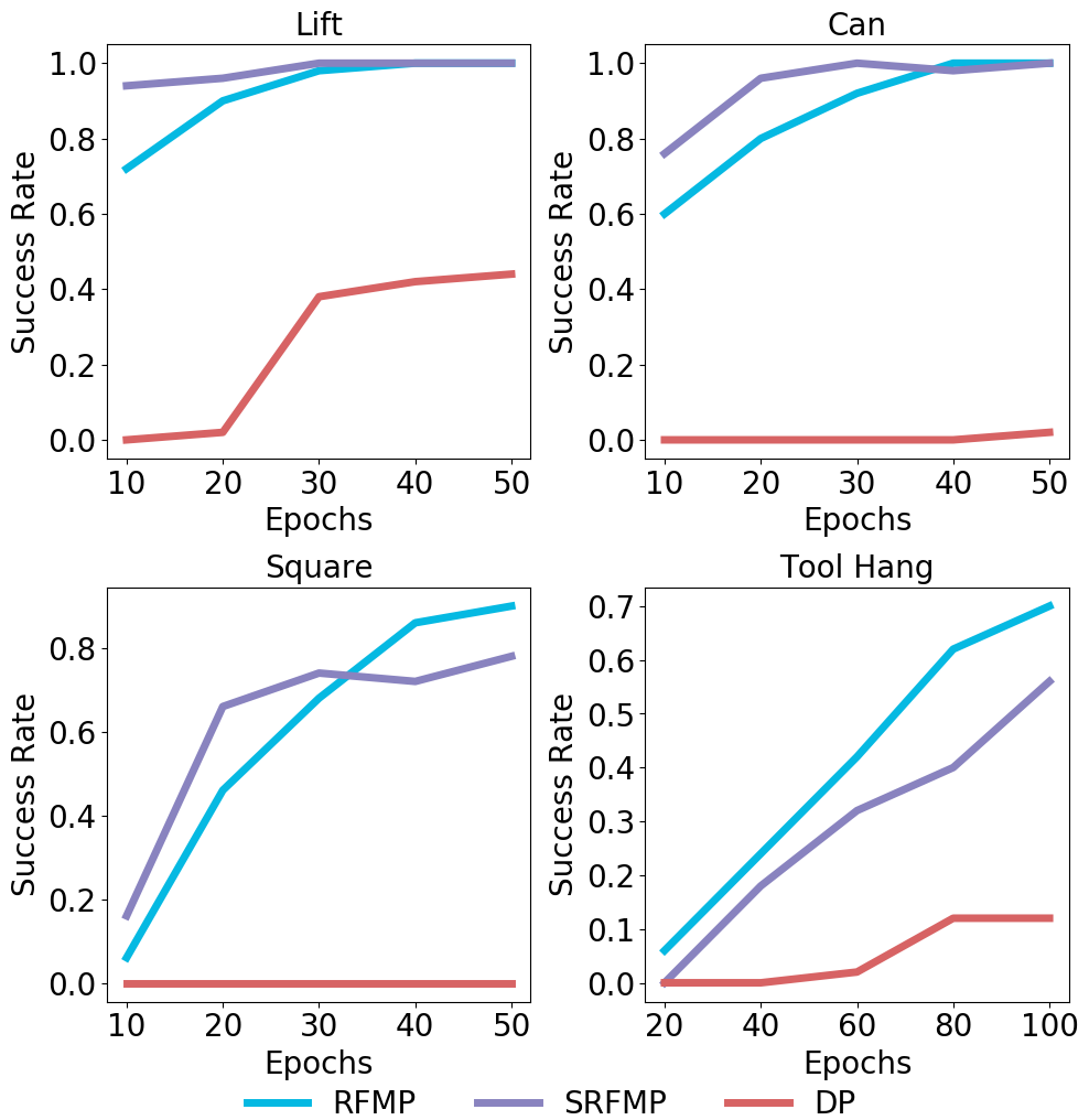
图 6:在不同检查点下基于状态观察的 Robomimic 任务的成功率。Lift、Can 和 Square 任务的模型性能在整个 50 -epoch 训练过程中每 10 个 epoch 使用 3 NFE 进行检查。对于 Tool Hang 任务,模型在 100 个 epoch 上进行训练,并在每 20 个 epoch 使用 10 NFE 进行检查。
V-C1State-based Observations
V-C1 基于状态的观察
We first assess the training efficiency of RFMP and SRFMP and compare it against DP by analyzing their performance at different training stages. Figure 6 shows the success rate of the three policies as a function of the number of training epochs for each task. All policies are evaluated with 3 NFE for Lift, Can, and Square, and with 10 NFE for Tool Hang. We observe that RFMP and SRFMP consistently outperform DP across all tasks, requiring fewer training epochs to achieve comparable or superior performance. For the easier tasks (Lift and Can), both RFMP and SRFMP achieve high performance after just 20 training epochs, while the success rate of DP remains low after 50 epochs. This trend persists in the harder tasks (Square and Tool Hang), with RFMP and SRFMP reaching high success rates significantly faster than DP.
我们首先评估了 RFMP 和 SRFMP 的训练效率,并通过分析它们在不同训练阶段的表现,将其与 DP 进行比较。图 6 显示了三种策略在每个任务的训练周期数与成功率的关系。所有策略在 Lift、Can 和 Square 任务中使用 3 NFE 进行评估,在 Tool Hang 任务中使用 10 NFE 进行评估。我们观察到,RFMP 和 SRFMP 在所有任务中始终优于 DP,所需的训练周期更少,但能达到相当或更好的性能。对于较简单的任务(Lift 和 Can),RFMP 和 SRFMP 在仅仅 20 个训练周期后就能达到高性能,而 DP 在 50 个周期后成功率仍然较低。这一趋势在较难的任务(Square 和 Tool Hang)中也持续存在,RFMP 和 SRFMP 比 DP 更快地达到高成功率。
表 VII:基于状态的 Robomimic 任务中不同 NFE 值的成功率。
| Task 任务 | Lift 提升 | Can 能 | Square 正方形 | Tool Hang 工具挂起 | ||||||||||||||||
|---|---|---|---|---|---|---|---|---|---|---|---|---|---|---|---|---|---|---|---|---|
| NFE | 1 | 2 | 3 | 5 | 10 | 1 | 2 | 3 | 5 | 10 | 1 | 2 | 3 | 5 | 10 | 1 | 2 | 3 | 5 | 10 |
| RFMP | 𝟏 | 𝟏 | 𝟏 | 0.98 | 𝟏 | 0.96 | 𝟏 | 𝟏 | 0.98 | 0.96 | 0.78 | 0.82 | 0.9 | 0.84 | 0.9 | 0.16 | 0.3 | 0.36 | 0.56 | 0.7 |
| SRFMP | 𝟏 | 𝟏 | 𝟏 | 𝟏 | 𝟏 | 0.94 | 0.96 | 𝟏 | 0.98 | 0.98 | 0.72 | 0.7 | 0.78 | 0.7 | 0.72 | 0.26 | 0.2 | 0.28 | 0.5 | 0.56 |
| DP | 0 | 0.78 | 0.96 | 0.96 | 0.98 | 0 | 0.38 | 0.82 | 0.92 | 0.9 | 0 | 0.4 | 0.62 | 0.66 | 0.66 | 0 | 0 | 0.04 | 0.1 | 0.08 |
表 VIII:基于状态观察的 robomimic 任务中不同 NFE 的预测机器人轨迹的抖动性。所有值均以千为单位表示,值越低,预测越平滑。
| Task | Lift 提升 | Can 能 | Square 正方形 | Tool Hang 工具挂起 | ||||||||||||||||
|---|---|---|---|---|---|---|---|---|---|---|---|---|---|---|---|---|---|---|---|---|
| NFE | 1 | 2 | 3 | 5 | 10 | 1 | 2 | 3 | 5 | 10 | 1 | 2 | 3 | 5 | 10 | 1 | 2 | 3 | 5 | 10 |
| RFMP | 9.75 | 8.82 | 9.05 | 8.82 | 8.44 | 7.92 | 6.62 | 6.59 | 6.45 | 9.68 | 9.11 | 6.39 | 5.49 | 5.3 | 4.29 | 4.43 | 3.98 | 4.54 | 5.25 | 4.79 |
| SRFMP | 10.2 | 10.1 | 7.79 | 9.75 | 9.35 | 7.6 | 7.75 | 6.35 | 7.16 | 6.86 | 9.29 | 9.67 | 6.59 | 8.3 | 7.81 | 5.48 | 5.0 | 5.33 | 6.28 | 6.29 |
| DP | 344 | 14.4 | 8.15 | 7.3 | 8.57 | 558 | 19.9 | 6.94 | 5.93 | 6.19 | 558 | 19.9 | 7.28 | 14.7 | 5.48 | 777 | 9.42 | 9.95 | 5.39 | 7.41 |
Next, we evaluate the performance of the policies for different NFE in the testing phase. For RFMP and SRFMP, we use the 50-epoch models for Lift, Can, and Square, and the 100-epoch model for Tool Hang. DP is further trained for a total of 300 epochs and we select the model at the best validation epoch. The results are reported in Table VII. RFMP and SRFMP outperform DP for all task and all NFE, even though DP was trained for more epochs. Moreover, we observe that RFMP and SRFMP are generally more robust to low NFE than DP. They achieve 100% success rate at almost all NFE values for the easier Lift and Can tasks, while DP’s performance drastically drops for 1 and 2 NFE. We observe a similar trend for the Square task, where the performance of RFMP and SRFMP slightly improves when increasing the NFE. The performance of all models drops for Tool Hang, which is the most complex of the considered tasks. In this case, the performance of RFMP and SRFMP is limited for low NFE values and improves for higher NFE. DP performs poorly for all considered NFE values. Table VIII reports the jerkiness as a measure of the smoothness of the trajectories generated by the different policies. We observe that RFMP and SRFMP produce arguably smoother trajectories than DP for low NFE, as indicated by the lower jerkiness values. The smoothness of the trajectories becomes comparable for higher NFE. In summary, both RFMP and SRFMP achieve high success rates and smooth action predictions with low NFE, enabling faster inference without compromising task completion.
接下来,我们评估不同 NFE 在测试阶段的策略性能。对于 RFMP 和 SRFMP,我们使用 50 轮次模型进行 Lift、Can 和 Square 任务,并使用 100 轮次模型进行 Tool Hang 任务。DP 进一步训练了总共 300 轮次,并选择了最佳验证轮次的模型。结果如表 VII 所示。RFMP 和 SRFMP 在所有任务和所有 NFE 上都优于 DP,即使 DP 训练了更多轮次。此外,我们观察到 RFMP 和 SRFMP 通常比 DP 对低 NFE 更具鲁棒性。它们在几乎所有 NFE 值上都能在较简单的 Lift 和 Can 任务中达到 100 %的成功率,而 DP 的性能在 1 和 2 NFE 时急剧下降。我们在 Square 任务中观察到类似的趋势,随着 NFE 的增加,RFMP 和 SRFMP 的性能略有提高。所有模型在 Tool Hang 任务中的性能下降,这是所考虑任务中最复杂的。在这种情况下,RFMP 和 SRFMP 在低 NFE 值时的性能有限,但在较高 NFE 时有所提高。DP 在所有考虑的 NFE 值上表现不佳。 表八报告了不同策略生成的轨迹平滑度的抖动性。我们观察到,RFMP 和 SRFMP 在低 NFE 时产生的轨迹比 DP 更平滑,如较低的抖动值所示。轨迹的平滑度在较高 NFE 时变得相当。总之,RFMP 和 SRFMP 都在低 NFE 下实现了高成功率和平滑的动作预测,从而在不影响任务完成的情况下实现了更快的推理。
V-C2Vision-based Observations
V-C2 基于视觉的观察
Next, we assess our models performance when the vector field is conditioned on visual observations. We consider the tasks Lift, Can and Square with the same policy settings and networks (see Table I). Each observation 𝒐s at time s corresponds to the embeddings vector obtained from an image of an over-the-shoulder camera and an image of an in-hand camera. We train the models for a total 100 epochs and use the best-performing checkpoint for evaluation. The performance of different policies is reported in Table IX. RFMP and SRFMP consistently outperform DP on all tasks, regardless of the NFE. As for the previous experiments, our models are remarkably robust to changes in NFE compared to DP. Importantly, SRFMP consistently surpassed RFMP for 1 and 2 NFE. Regarding Can and Square tasks, SRFMP with 1 NFE achieved performance on par with RFMP using 3 NFE. This efficiency gain showcases the benefits of enhancing the policies with stability to the target distribution for reducing their inference time. We additionally compare RFMP and SRFMP against CP by reporting the performance obtained from [3] in Table IX. Our models achieve a competitive performance compared to CP, which is a method aimed at steeping up inference. However, in contrast to CP, our models are easy and fast to train.
接下来,我们评估在向量场以视觉观测为条件时模型的性能。我们考虑了 Lift、Can 和 Square 任务,使用相同的策略设置和网络(见表)。每个时间点的观测值对应于从肩上摄像头和手持摄像头的图像中获得的嵌入向量。我们训练模型共 100 个周期,并使用表现最好的检查点进行评估。不同策略的性能报告在表 IX 中。RFMP 和 SRFMP 在所有任务上始终优于 DP,无论 NFE 如何变化。与之前的实验一样,我们的模型在 NFE 变化方面比 DP 显著更稳健。重要的是,SRFMP 在 1 和 2 NFE 上始终超过 RFMP。关于 Can 和 Square 任务,SRFMP 在 1 NFE 上的表现与 RFMP 在 3 NFE 上的表现相当。这种效率提升展示了通过增强策略对目标分布的稳定性来减少推理时间的好处。我们还通过报告表 IX 中 [3] 获得的性能来比较 RFMP 和 SRFMP 与 CP 的表现。 我们的模型与 CP 相比表现出竞争力,CP 是一种旨在加速推理的方法。然而,与 CP 相比,我们的模型易于训练且训练速度快。
表 IX:基于视觉的 robomimic 任务中成功率与 NFE 的函数关系。CP 结果对应于[3]中报告的结果。
| Task 任务 | Lift 提升 | Can 能 | Square 正方形 | ||||||||||||
|---|---|---|---|---|---|---|---|---|---|---|---|---|---|---|---|
| NFE | NFE | NFE | |||||||||||||
| Policy 政策 | 1 | 2 | 3 | 5 | 10 | 1 | 2 | 3 | 5 | 10 | 1 | 2 | 3 | 5 | 10 |
| RFMP | 𝟏 | 𝟏 | 𝟏 | 𝟏 | 𝟏 | 0.78 | 0.82 | 0.9 | 0.96 | 0.94 | 0.56 | 0.74 | 0.9 | 0.9 | 0.9 |
| SRFMP | 𝟏 | 𝟏 | 𝟏 | 𝟏 | 𝟏 | 0.88 | 0.88 | 0.9 | 0.9 | 0.86 | 0.86 | 0.82 | 0.9 | 0.88 | 0.9 |
| DP | 0 | 0.7 | 0.96 | 0.98 | 0.98 | 0 | 0.38 | 0.66 | 0.68 | 0.66 | 0 | 0.04 | 0.16 | 0.26 | 0.12 |
| CP | 1¯ | N.A. | 1¯ | N.A. | N.A. | 0.98¯ | N.A. | 0.95¯ | N.A. | N.A. | 0.92¯ | N.A. | 0.96¯ | N.A. | N.A. |
V-DReal Robotic Experiments
V-D 真实机器人实验
Finally, we evaluate RFMP and SRFMP on two real-world tasks, namely Pick & Place and Mug Flipping, with a 7-DoF robotic manipulator.
最后,我们在两个实际任务中评估了 RFMP 和 SRFMP,即拾取和放置以及翻转杯子,使用 7 自由度的机器人操纵器。
V-D1Experimental Setup V-D1 实验设置
Figure 7 shows our experimental setup. The tasks are performed on a Franka Emika Panda robot arm. We collect the demonstrations via a teleoperation system consisting of two robot twins. Demonstrations are collected by an expert who guides the source robot. All the demonstrations were recorded in a fairly controlled environment with minimal variation in lighting and background. The target robot then reads the end-effector pose of the source robot and reproduces it via a Cartesian impedance controller. Each observation 𝒐s is composed of the end-effector position, and of the image embedding obtained from the ResNet vision backbone that processes the images from an over-the-shoulder camera. The policies are trained to generate 8-dimensional actions composed of the position, orientation, and gripper state.
图 7 显示了我们的实验设置。任务是在 Franka Emika Panda 机器人手臂上执行的。我们通过由两个机器人双胞胎组成的远程操作系统收集演示。演示由专家收集,专家引导源机器人。所有演示都在光照和背景变化最小的受控环境中记录。目标机器人然后读取源机器人的末端执行器姿态,并通过笛卡尔阻抗控制器再现它。每个观测 𝒐s 由末端执行器位置和从 ResNet 视觉主干处理的肩膀上方摄像头图像嵌入组成。策略被训练生成 8 维动作,由位置、方向和夹持器状态组成。
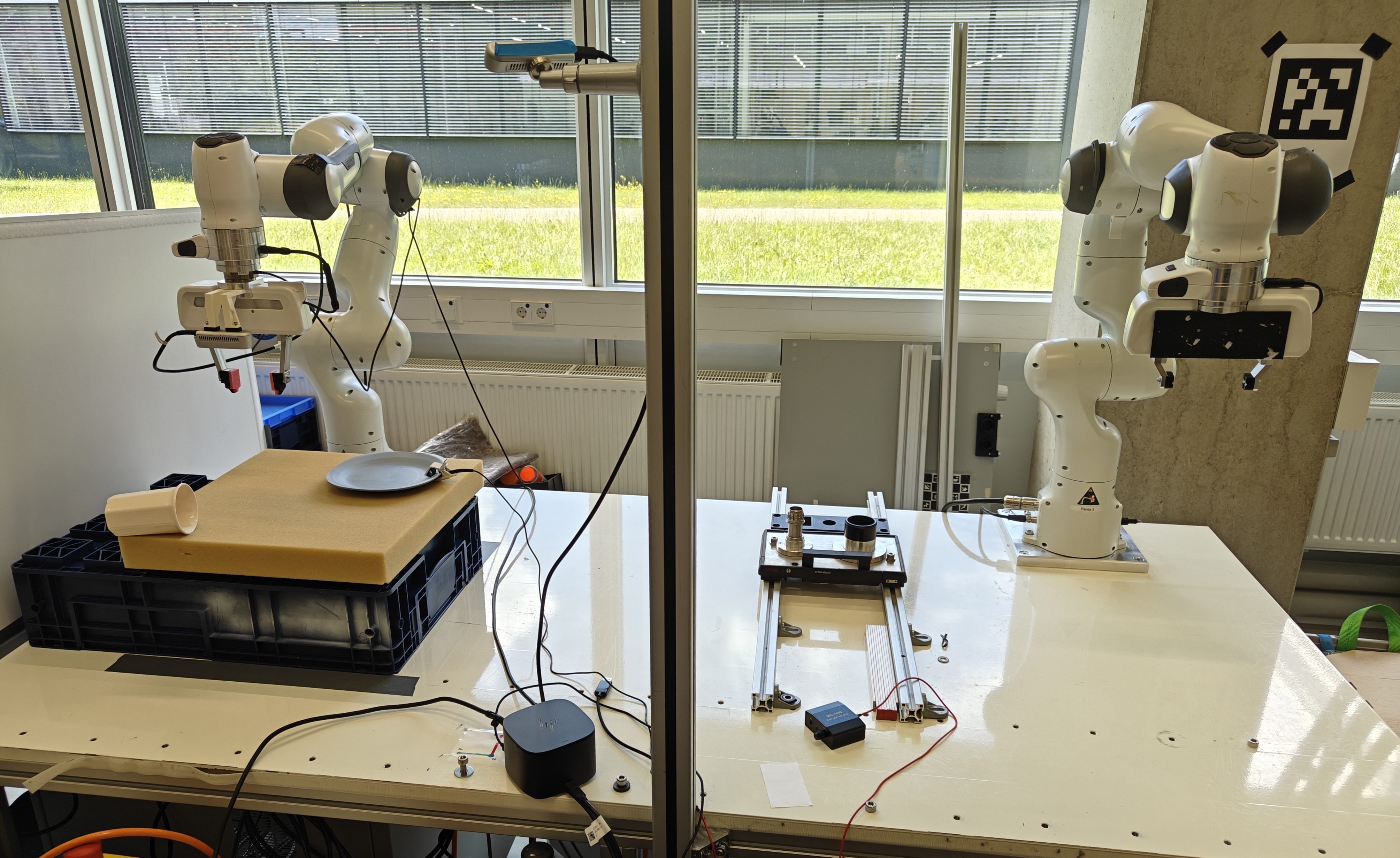
图 7:机器人实验设置包括 2 个 Franka Emika Panda 机器人手臂用于远程操作和一个肩膀上的摄像头(Realsense d435)。左臂是跟随机器人,而右臂作为领导者。在教学阶段,人类专家控制领导者手臂通过 ROS 向跟随机器人发送所需的参考。在测试期间,只有跟随手臂在运行。
V-D2Pick & Place V-D2 拣选与放置
The goal of this task is to test the ability of RFMP and SRFMP to learn Euclidean policies in real-world settings. The task consists of approaching and picking up a white mug, and to then place it on a pink plate, as shown in Figure 8. Note that the end effector of the robot points downwards during the entire task, so that its orientation remains almost constant.
这个任务的目标是测试 RFMP 和 SRFMP 在现实环境中学习欧几里得策略的能力。任务包括接近并拿起一个白色的杯子,然后将其放在一个粉红色的盘子上,如图 8 所示。请注意,机器人的末端执行器在整个任务过程中都指向下方,因此其方向几乎保持不变。
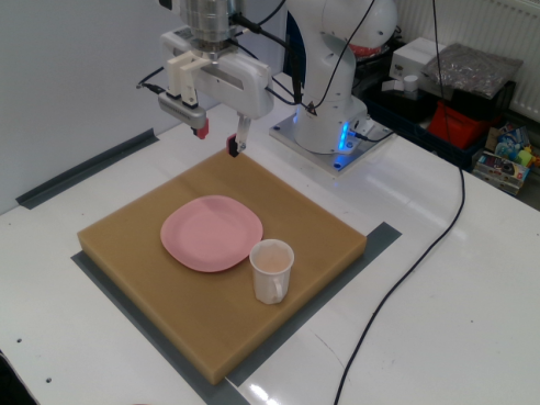
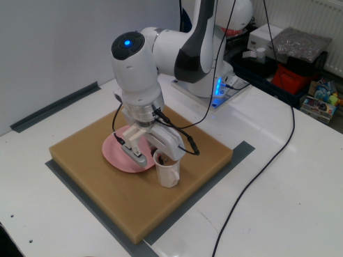
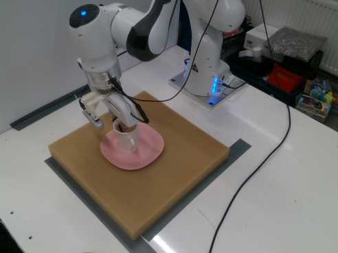
图 8:拾取和放置:首先,机器人末端执行器接近并抓住白色杯子。然后,它抬起杯子并将其直立放置在粉红色盘子上。
We collect 100 demonstrations where the white mug is randomly placed on the yellow mat, while the pink plate position and end-effector initial position are slightly varied. We split our demonstration data to use 90 demonstrations for training and 10 for validation. All models are trained for 300 epochs with the same training hyperparameters as reported in Table I. As in previous experiments, we use the best-performing checkpoints of each model for evaluation.
我们收集了 100 次演示,其中白色杯子随机放置在黄色垫子上,而粉红色盘子的位置和末端执行器的初始位置略有变化。我们将演示数据分为 90 次用于训练, 10 次用于验证。所有模型都在 300 个周期内使用表中报告的相同训练超参数进行训练。与之前的实验一样,我们使用每个模型表现最好的检查点进行评估。
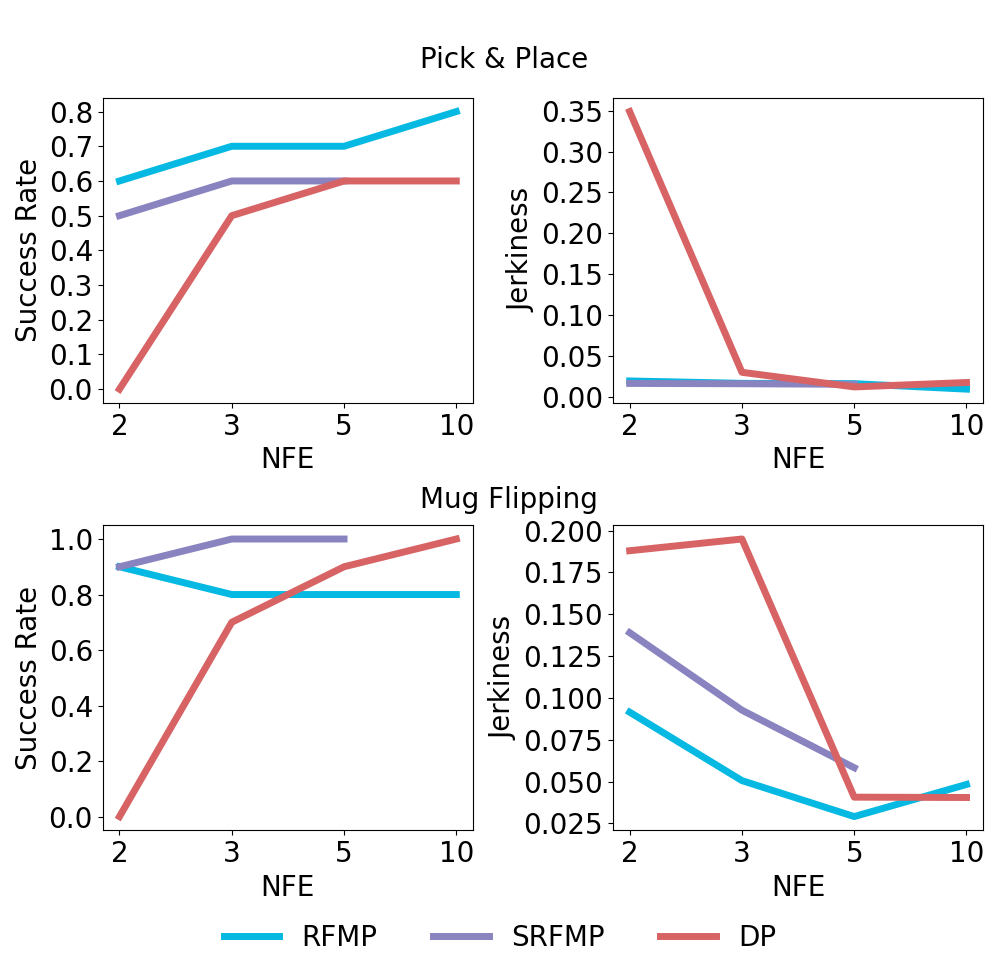
图 9:在拾取和放置以及翻转杯子任务中,成功率和预测动作的抖动性随 NFE 的变化。
During testing, we systematically place the white mug at 10 different locations on a semi-grid covering the surface of the yellow sponge. We evaluate the performance of RFMP, SRFMP, and DP as a function of different NFE values, under two metrics: Success rate and prediction smoothness. Figure 9 shows the increased robustness of RFMP and SRFMP to NFE compared to DP. Notably, DP requires more NFEs to achieve a success rate competitive to RFMP and SRFMP, which display high performance with only 2 NFE. Moreover, DP generated highly jerky predictions when using 2 NFE. In contrast, RFMP and SRFMP consistently retrieve smooth trajectories, regardless of the NFE.
在测试过程中,我们系统地将白色杯子放置在覆盖黄色海绵表面的半网格的 10 个不同位置。我们评估了 RFMP、SRFMP 和 DP 在不同 NFE 值下的性能,使用两个指标:成功率和预测平滑度。图 9 显示了 RFMP 和 SRFMP 相比 DP 对 NFE 的增强鲁棒性。值得注意的是,DP 需要更多的 NFE 才能达到与 RFMP 和 SRFMP 竞争的成功率,而 RFMP 和 SRFMP 仅用 2 个 NFE 就表现出高性能。此外,DP 在使用 2 个 NFE 时生成了非常不稳定的预测。相比之下,RFMP 和 SRFMP 无论 NFE 如何,都能始终检索到平滑的轨迹。
Our experiments also revealed that slight variations in background and lighting conditions (e.g., cloudy and sunny days), had minimal impact on the policies performance. However, consistent failures were observed when the mug was initially positioned on the right side of the yellow mat, where the robot often obstructs the external camera view when approaching the mug. A multi-camera setting may improve performance on such occlusion cases.
我们的实验还发现,背景和光照条件的轻微变化(例如,多云和晴天)对策略性能的影响很小。然而,当杯子最初放置在黄色垫子右侧时,常常会出现一致的失败情况,因为机器人在接近杯子时经常会遮挡外部摄像头的视野。多摄像头设置可能会改善这种遮挡情况的性能。
V-D3Mug Flipping V-D3 杯子翻转
In this task, a white mug is initially positioned horizontally on a yellow sponge, as shown in Figure 10. The task consists of two stages: First, the robot locates the white mug and grasps it by rotating its end-effector to align with the mug orientation. The robot then places the mug upright on the blue plate. Note that this task demands the robot to execute elaborated rotation trajectories for both grasping and placing. For this task, we collect 50 demonstrations with the white mug randomly positioned and rotated on the left side of a yellow sponge. Note that we use only the left side as the task requires the robot to operate near its workspace limits, which are prohibitive when the mug is placed on the right side. Furthermore, the end-effector initial pose was also slightly varied across the demonstrations. The policy hyperparameters for this task are provided in Table I.
在这个任务中,如图 10 所示,白色杯子最初水平放置在黄色海绵上。任务分为两个阶段:首先,机器人定位白色杯子,并通过旋转末端执行器使其与杯子方向对齐来抓取杯子。然后,机器人将杯子直立放置在蓝色盘子上。请注意,此任务要求机器人在抓取和放置时执行复杂的旋转轨迹。对于此任务,我们收集了 50 次演示,白色杯子随机放置并旋转在黄色海绵的左侧。请注意,我们仅使用左侧,因为任务要求机器人在其工作空间极限附近操作,当杯子放置在右侧时,这将是不可行的。此外,演示过程中末端执行器的初始姿态也略有变化。此任务的策略超参数见表。
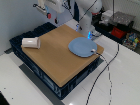
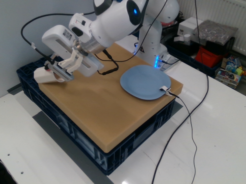
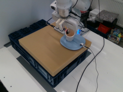
图 10:杯子翻转:机器人旋转其末端执行器以对齐白色杯子的方向,然后抓住它。然后将杯子直立放在蓝色盘子上。
Figure 9 shows the results of evaluating the different considered policies using the same two metrics as the Pick & Place task, namely success rate and trajectory smoothness. Both RFMP and SRFMP are significantly more robust to different NFE in terms of success rate when compared to DP. While the smoothness of RFMP and SRFMP is slightly affected by NFE in this particular task, both methods still outperform DP in this regard. Similarly to the Pick & Place, slight variations on lightning and background had a negligible effect on the performance of the tested policies.
图 9 显示了使用与 Pick & Place 任务相同的两个指标(即成功率和轨迹平滑度)评估不同考虑的策略的结果。与 DP 相比,RFMP 和 SRFMP 在成功率方面对不同的 NFE 显著更具鲁棒性。虽然在这个特定任务中,NFE 对 RFMP 和 SRFMP 的平滑度有轻微影响,但这两种方法在这方面仍优于 DP。与 Pick & Place 类似,光照和背景的轻微变化对测试策略的性能影响可以忽略不计。
In summary, our findings from both simulated and real-world tasks show that RFMP and SRFMP offer significant advantages over DP. In particular, RFMP and SRFMP achieve faster inference by using fewer NFE without compromising success rates regardless of the observation type. This translates into highly-robust visuomotor policies. Importantly, these advantages do not come at the cost of elaborated training strategies like those used in consistency-based models. In fact, our models demonstrate competitive performance against CP, while being notably easier to train. Regarding the difference between SRFMP and RFMP, the results did not show significant performance gains in terms of success rate and prediction smoothness. Nevertheless, SRFMP shows to be easier to train, achieving higher success rate than RFMP for fewer training epochs (e.g., in Lift, Can, Square tasks).
总之,我们在模拟和现实任务中的发现表明,RFMP 和 SRFMP 相对于 DP 具有显著优势。特别是,RFMP 和 SRFMP 通过使用更少的 NFE 实现了更快的推理,而不会影响成功率,无论观察类型如何。这转化为高度鲁棒的视觉运动策略。重要的是,这些优势并不需要像一致性模型那样复杂的训练策略。事实上,我们的模型在与 CP 的竞争中表现出色,同时训练起来明显更容易。关于 SRFMP 和 RFMP 之间的差异,结果并未显示在成功率和预测平滑度方面的显著性能提升。然而,SRFMP 显示出更容易训练,在更少的训练周期内(例如,在 Lift、Can、Square 任务中)实现了比 RFMP 更高的成功率。
VIConclusion VI 结论
This paper introduced Stable Riemannian Flow Matching Policy (SRFMP), a novel framework that combines the easy training of flow matching with stability-based robustness properties for visuomotor policy learning. SRFMP builds on our extension of stable flow matching to Riemannian manifolds, providing stable convergence of the learned flow to the support of Riemannian target distributions. Our simulated and real-world experiments show that both our previous work on RFMP and its stable counterpart SRFMP outperform diffusion policies and achieve comparable performance to recent distillation-based extensions, while offering advantages in terms of inference speed, ease of training, and robust performance even with limited NFEs and training epochs. Future work will focus on exploring equivariant policy structures to potentially reduce the number of required demonstrations and to improve generalization. Additionally, we aim to investigate multi-modal perception backbones for tackling contact-rich tasks.
本文介绍了稳定黎曼流匹配策略(SRFMP),这是一个结合了流匹配的易训练性和基于稳定性的鲁棒性特性的视觉运动策略学习的新框架。SRFMP 基于我们将稳定流匹配扩展到黎曼流形的工作,提供了学习流向黎曼目标分布支持的稳定收敛。我们的模拟和现实世界实验表明,我们之前的 RFMP 工作及其稳定的对应物 SRFMP 都优于扩散策略,并在推理速度、训练容易性和即使在有限的 NFE 和训练周期下也能表现出鲁棒性能方面,达到了与最近基于蒸馏的扩展相当的性能。未来的工作将重点探索等变策略结构,以可能减少所需示范的数量并提高泛化能力。此外,我们还旨在研究多模态感知骨干,以应对接触丰富的任务。
References 参考文献
- [1]↑J. Urain, A. Mandlekar, Y. Du, M. Shafiullah, D. Xu, K. Fragkiadaki, G. Chalvatzaki, and J. Peters, “Deep generative models in robotics: A survey on learning from multimodal demonstrations,” arXiv preprint arXiv:2408.04380, 2024.
- [2]↑C. Chi, S. Feng, Y. Du, Z. Xu, E. Cousineau, B. Burchfiel, and S. Song, “Diffusion policy: Visuomotor policy learning via action diffusion,” in Robotics: Science and Systems (R:SS), 2023.
- [3]↑A. Prasad, K. Lin, J. Wu, L. Zhou, and J. Bohg, “Consistency policy: Accelerated visuomotor policies via consistency distillation,” in Robotics: Science and Systems (R:SS), 2024.
A. Prasad, K. Lin, J. Wu, L. Zhou, and J. Bohg, “一致性策略:通过一致性蒸馏加速视觉运动策略,” 载于《机器人:科学与系统 (R:SS)》,2024 年. - [4]↑M. Reuss, M. Li, X. Jia, and R. Lioutikov, “Goal-conditioned imitation learning using score-based diffusion policies,” in Robotics: Science and Systems (R:SS), 2023.
- [5]↑S.-F. Chen, H.-C. Wang, M.-H. Hsu, C.-M. Lai, and S.-H. Sun, “Diffusion model-augmented behavioral cloning,” in Intl. Conf. on Machine Learning (ICML), 2024.
- [6]↑Y. Ze, G. Zhang, K. Zhang, C. Hu, M. Wang, and H. Xu, “3d diffusion policy: Generalizable visuomotor policy learning via simple 3d representations,” in Robotics: Science and Systems (R:SS), 2024.
- [7]↑J. Yang, Z. Cao, C. Deng, R. Antonova, S. Song, and J. Bohg, “Equibot: SIM(3)-equivariant diffusion policy for generalizable and data efficient learning,” in Conference on Robot Learning (CoRL), 2024.
J. Yang, Z. Cao, C. Deng, R. Antonova, S. Song, and J. Bohg, “Equibot: SIM(3)-等变扩散策略用于可推广和数据高效学习,” in Conference on Robot Learning (CoRL), 2024. - [8]↑P. Florence, C. Lynch, A. Zeng, O. A. Ramirez, A. Wahid, L. Downs, A. Wong, J. Lee, I. Mordatch, and J. Tompson, “Implicit behavioral cloning,” in Conference on Robot Learning (CoRL), ser. Proceedings of Machine Learning Research, vol. 164. PMLR, 2022, pp. 158–168.
- [9]↑N. M. Shafiullah, Z. Cui, A. A. Altanzaya, and L. Pinto, “Behavior transformers: Cloning k modes with one stone,” in Neural Information Processing Systems (NeurIPS), 2022.
N. M. Shafiullah, Z. Cui, A. A. Altanzaya, and L. Pinto, “行为变换器:一石克隆 k 模式,” in 神经信息处理系统 (NeurIPS), 2022. - [10]↑A. Mandlekar, D. Xu, J. Wong, S. Nasiriany, C. Wang, R. Kulkarni, L. Fei-Fei, S. Savarese, Y. Zhu, and R. Martín-Martín, “What matters in learning from offline human demonstrations for robot manipulation,” in Conference on Robot Learning (CoRL), 2022, pp. 1678–1690.
- [11]↑C. Luo, “Understanding diffusion models: A unified perspective,” arXiv preprint arXiv2208.11970, 2022.
- [12]↑J. Ho, A. Jain, and P. Abbeel, “Denoising diffusion probabilistic models,” Advances in neural information processing systems, vol. 33, pp. 6840–6851, 2020.
- [13]↑J. Song, C. Meng, and S. Ermon, “Denoising diffusion implicit models,” in Intl. Conf. on Learning Representations (ICLR), 2020.
- [14]↑C.-W. Huang, M. Aghajohari, J. Bose, P. Panangaden, and A. Courville, “Riemannian diffusion models,” in Neural Information Processing Systems (NeurIPS), 2022.
C.-W. Huang, M. Aghajohari, J. Bose, P. Panangaden, and A. Courville, “黎曼扩散模型,” in Neural Information Processing Systems (NeurIPS), 2022. - [15]↑Y. Lipman, R. T. Chen, H. Ben-Hamu, M. Nickel, and M. Le, “Flow matching for generative modeling,” in Intl. Conf. on Learning Representations (ICLR), 2022.
- [16]↑R. T. Chen and Y. Lipman, “Riemannian flow matching on general geometries,” in Intl. Conf. on Learning Representations (ICLR), 2023.
R. T. Chen 和 Y. Lipman, “一般几何上的黎曼流匹配,” 2023 年国际学习表征会议 (ICLR). - [17]↑M. Braun, N. Jaquier, L. Rozo, and T. Asfour, “Riemannian flow matching policy for robot motion learning,” in IEEE/RSJ Intl. Conf. on Intelligent Robots and Systems (IROS), 2024.
- [18]↑A. Lemme, Y. Meirovitch, M. Khansari-Zadeh, T. Flash, A. Billard, and J. J. Steil, “Open-source benchmarking for learned reaching motion generation in robotics,” Paladyn, Journal of Behavioral Robotics, vol. 6, no. 1, 2015.
A. Lemme, Y. Meirovitch, M. Khansari-Zadeh, T. Flash, A. Billard, and J. J. Steil, “开源基准测试用于机器人学习到的到达运动生成,” Paladyn, 行为机器人学杂志, 第 6 卷, 第 1 期, 2015 年. - [19]↑C. I. Sprague, A. Elofsson, and H. Azizpour, “Stable autonomous flow matching,” arXiv preprint arXiv2402.05774, 2024.
- [20]↑S. Christopher Iliffe, E. Arne, and A. Hossein, “Incorporating stability into flow matching,” in ICML 2024 Workshop on Structured Probabilistic Inference & Generative Modeling, 2024.
S. Christopher Iliffe, E. Arne, 和 A. Hossein, “将稳定性纳入流匹配,” 载于 ICML 2024 结构化概率推理与生成建模研讨会, 2024. - [21]↑J. LaSalle, “Some extensions of Liapunov’s second method,” IRE Transactions on Circuit Theory, vol. 7, no. 4, pp. 520–527, 1960.
- [22]↑G. Papamakarios, E. Nalisnick, D. J. Rezende, S. Mohamed, and B. Lakshminarayanan, “Normalizing flows for probabilistic modeling and inference,” Journal of Machine Learning Research, vol. 22, no. 57, pp. 1–64, 2021.
- [23]↑M. A. Rana, A. Li, D. Fox, B. Boots, F. Ramos, and N. Ratliff, “Euclideanizing flows: Diffeomorphic reduction for learning stable dynamical systems,” in Learning for Dynamics and Control. PMLR, 2020, pp. 630–639.
- [24]↑S. A. Khader, H. Yin, P. Falco, and D. Kragic, “Learning stable normalizing-flow control for robotic manipulation,” in 2021 IEEE International Conference on Robotics and Automation (ICRA). IEEE, 2021, pp. 1644–1650.
- [25]↑J. Urain, M. Ginesi, D. Tateo, and J. Peters, “Imitationflow: Learning deep stable stochastic dynamic systems by normalizing flows,” in 2020 IEEE/RSJ International Conference on Intelligent Robots and Systems (IROS). IEEE, 2020, pp. 5231–5237.
J. Urain, M. Ginesi, D. Tateo, 和 J. Peters, “Imitationflow: Learning deep stable stochastic dynamic systems by normalizing flows,” 见 2020 IEEE/RSJ International Conference on Intelligent Robots and Systems (IROS). IEEE, 2020, 第 5231–5237 页. - [26]↑J. Urain, D. Tateo, and J. Peters, “Learning stable vector fields on lie groups,” IEEE Robotics and Automation Letters, vol. 7, no. 4, pp. 12 569–12 576, 2022.
- [27]↑J. Zhang, H. B. Mohammadi, and L. Rozo, “Learning Riemannian stable dynamical systems via diffeomorphisms,” in 6th Annual Conference on Robot Learning, 2022.
张杰, H. B. Mohammadi, 和 L. Rozo, “通过微分同胚学习黎曼稳定动力系统,” 在第六届机器人学习年会, 2022. - [28]↑L. Yang, Z. Zhang, Y. Song, S. Hong, R. Xu, Y. Zhao, W. Zhang, B. Cui, and M.-H. Yang, “Diffusion models: A comprehensive survey of methods and applications,” ACM Comput. Surv., vol. 56, no. 4, 2023.
- [29]↑M. Janner, Y. Du, J. B. Tenenbaum, and S. Levine, “Planning with diffusion for flexible behavior synthesis,” in Intl. Conf. on Machine Learning (ICML), 2022.
- [30]↑Z. Wang, J. J. Hunt, and M. Zhou, “Diffusion policies as an expressive policy class for offline reinforcement learning,” in Intl. Conf. on Learning Representations (ICLR), 2023.
- [31]↑Y. Song, P. Dhariwal, M. Chen, and I. Sutskever, “Consistency models,” in Intl. Conf. on Machine Learning (ICML). PMLR, 2023, pp. 32 211–32 252.
- [32]↑G. Lu, Z. Gao, T. Chen, W. Dai, Z. Wang, and Y. Tang, “Manicm: Real-time 3d diffusion policy via consistency model for robotic manipulation,” arXiv preprint arXiv:2406.01586, 2024.
- [33]↑Z. Wang, Z. Li, A. Mandlekar, Z. Xu, J. Fan, Y. Narang, L. Fan, Y. Zhu, Y. Balaji, M. Zhou et al., “One-step diffusion policy: Fast visuomotor policies via diffusion distillation,” arXiv preprint arXiv:2410.21257, 2024.
Z. Wang, Z. Li, A. Mandlekar, Z. Xu, J. Fan, Y. Narang, L. Fan, Y. Zhu, Y. Balaji, M. Zhou 等人,“一步扩散策略:通过扩散蒸馏实现快速视觉运动策略”,arXiv 预印本 arXiv:2410.21257,2024。 - [34]↑A. Tong, K. Fatras, N. Malkin, G. Huguet, Y. Zhang, J. Rector-Brooks, G. Wolf, and Y. Bengio, “Improving and generalizing flow-based generative models with minibatch optimal transport,” Transactions on Machine Learning Research, 2024.
- [35]↑X. Liu, C. Gong, and Q. Liu, “Flow straight and fast: Learning to generate and transfer data with rectified flow,” in Intl. Conf. on Learning Representations (ICLR), 2022.
- [36]↑A. J. Bose, T. Akhound-Sadegh, K. Fatras, G. Huguet, J. Rector-Brooks, C.-H. Liu, A. C. Nica, M. Korablyov, M. Bronstein, and A. Tong, “SE(3)-stochastic flow matching for protein backbone generation,” in Intl. Conf. on Learning Representations (ICLR), 2023.
- [37]↑A. Davtyan, S. Sameni, and P. Favaro, “Efficient video prediction via sparsely conditioned flow matching,” in Proceedings of the IEEE/CVF International Conference on Computer Vision, 2023, pp. 23 263–23 274.
- [38]↑V. T. Hu, W. Yin, P. Ma, Y. Chen, B. Fernando, Y. M. Asano, E. Gavves, P. Mettes, B. Ommer, and C. G. M. Snoek, “Motion flow matching for human motion synthesis and editing,” arXiv preprint arXiv:2312.08895, 2023.
V. T. Hu, W. Yin, P. Ma, Y. Chen, B. Fernando, Y. M. Asano, E. Gavves, P. Mettes, B. Ommer, 和 C. G. M. Snoek, “Motion flow matching for human motion synthesis and editing,” arXiv preprint arXiv:2312.08895, 2023. - [39]↑X. Zhang, Y. Pu, Y. Kawamura, A. Loza, Y. Bengio, D. L. Shung, and A. Tong, “Trajectory flow matching with applications to clinical time series modeling,” in Neural Information Processing Systems (NeurIPS), 2024.
- [40]↑H. Lin, O. Zhang, H. Zhao, D. Jiang, L. Wu, Z. Liu, Y. Huang, and S. Z. Li, “PPFlow: Target-aware peptide design with torsional flow matching,” in Intl. Conf. on Machine Learning (ICML), 2024.
- [41]↑A. H. Liu, M. Le, A. Vyas, B. Shi, A. Tjandra, and W.-N. Hsu, “Generative pre-training for speech with flow matching,” in Intl. Conf. on Learning Representations (ICLR), 2024.
- [42]↑N. Funk, J. Urain, J. Carvalho, V. Prasad, G. Chalvatzaki, and J. Peters, “Actionflow: Efficient, accurate, and fast policies with spatially symmetric flow matching,” in R:SS workshop: Structural Priors as Inductive Biases for Learning Robot Dynamics, 2024.
- [43]↑Q. Rouxel, A. Ferrari, S. Ivaldi, and J.-B. Mouret, “Flow matching imitation learning for multi-support manipulation,” arXiv preprint arXiv:2407.12381, 2024.
- [44]↑E. Chisari, N. Heppert, M. Argus, T. Welschehold, T. Brox, and A. Valada, “Learning robotic manipulation policies from point clouds with conditional flow matching,” in Conference on Robot Learning (CoRL), 2024.
E. Chisari, N. Heppert, M. Argus, T. Welschehold, T. Brox, 和 A. Valada, “通过条件流匹配从点云中学习机器人操作策略,” 2024 年机器人学习会议 (CoRL). - [45]↑M. do Carmo, Riemannian Geometry. Birkhäuser Basel, 1992.
- [46]↑J. M. Lee, Introduction to Riemannian manifolds. Springer, 2018, vol. 2.
J. M. Lee, Riemannian 流形导论. Springer, 2018, 第 2 卷. - [47]↑P.-A. Absil, R. Mahony, and R. Sepulchre, Optimization Algorithms on Matrix Manifolds. Princeton University Press, 2007.
- [48]↑N. Boumal, An introduction to optimization on smooth manifolds. Cambridge University Press, 2023.
- [49]↑R. T. Chen, Y. Rubanova, J. Bettencourt, and D. K. Duvenaud, “Neural ordinary differential equations,” Advances in neural information processing systems, vol. 31, 2018.
- [50]↑K. Atkinson, An introduction to numerical analysis. John wiley & sons, 1991.
K. Atkinson, 数值分析导论. 约翰·威利父子公司, 1991. - [51]↑J. M. Selig, Geometric fundamentals of robotics. Springer Science & Business Media, 2007.
J. M. Selig, 《机器人几何基础》. 施普林格科学与商业媒体, 2007. - [52]↑F. Merat, “Introduction to robotics: Mechanics and control,” IEEE Journal on Robotics and Automation, vol. 3, no. 2, pp. 166–166, 1987.
- [53]↑X. Pennec, “Intrinsic statistics on Riemannian manifolds: Basic tools for geometric measurements,” Journal of Mathematical Imaging and Vision, vol. 25, p. 127–154, 2006.
- [54]↑F. Galaz-Garcia, M. Papamichalis, K. Turnbull, S. Lunagomez, and E. Airoldi, “Wrapped distributions on homogeneous Riemannian manifolds,” arXiv preprint arXiv:2204.09790, 2022.
- [55]↑D. Q. Mayne and H. Michalska, “Receding horizon control of nonlinear systems,” in IEEE Conference on Decision and Control (CDC), 1988, pp. 464–465.
D. Q. Mayne 和 H. Michalska,“非线性系统的递推控制”,在 IEEE 决策与控制会议 (CDC),1988 年,第 464-465 页。 - [56]↑J. P. La Salle, “An invariance principle in the theory of stability,” Tech. Rep., 1966.
J. P. La Salle, “稳定性理论中的不变性原理,” 技术报告, 1966. - [57]↑X. Mao, “Stochastic versions of the LaSalle theorem,” Journal of differential equations, vol. 153, no. 1, pp. 175–195, 1999.
X. Mao, “LaSalle 定理的随机版本,” 《微分方程杂志》, 第 153 卷, 第 1 期, 第 175-195 页, 1999 年. - [58]↑E. Perez, F. Strub, H. De Vries, V. Dumoulin, and A. Courville, “Film: Visual reasoning with a general conditioning layer,” in Proceedings of the AAAI conference on artificial intelligence, vol. 32, no. 1, 2018.
- [59]↑K. V. Mardia and P. E. Jupp, Distributions on Spheres. John Wiley and Sons, Ltd, 1999, ch. 9, pp. 159–192.
K. V. Mardia 和 P. E. Jupp,《球面上的分布》。John Wiley and Sons, Ltd,1999,第 9 章,第 159-192 页。 - [60]↑F. Galaz-Garcia, M. Papamichalis, K. Turnbull, S. Lunagomez, and E. Airoldi, “Wrapped distributions on homogeneous riemannian manifolds,” arXiv preprint arXiv:2204.09790, 2022.
- [61]↑I. Loshchilov and F. Hutter, “Decoupled weight decay regularization,” in Intl. Conf. on Learning Representations (ICLR), 2019.
I. Loshchilov 和 F. Hutter,“解耦权重衰减正则化”,发表于国际学习表征会议(ICLR),2019 年。 - [62]↑B. T. Polyak and A. B. Juditsky, “Acceleration of stochastic approximation by averaging,” SIAM journal on control and optimization, vol. 30, no. 4, pp. 838–855, 1992.
B. T. Polyak 和 A. B. Juditsky, “通过平均加速随机近似,” SIAM 控制与优化杂志, 第 30 卷, 第 4 期, 第 838–855 页, 1992. - [63]↑N. Jaquier, L. Rozo, and T. Asfour, “Unraveling the single tangent space fallacy: An analysis and clarification for applying Riemannian geometry in robot learning,” in IEEE Intl. Conf. on Robotics and Automation (ICRA), 2024, pp. 242–249.
N. Jaquier, L. Rozo, and T. Asfour, “揭开单切空间谬论:在机器人学习中应用黎曼几何的分析和澄清,” in IEEE Intl. Conf. on Robotics and Automation (ICRA), 2024, pp. 242–249.


 567
567

 被折叠的 条评论
为什么被折叠?
被折叠的 条评论
为什么被折叠?
 到【灌水乐园】发言


