sklearn中的异常检测方法

SKLEARN——Novelty and Outlier Detection

简介

     很多方法都可以检测一个新的检测样本，是符合当前样本分布的成员还是不一样的利群点。通常，这些方法被用来对真实数据集进行清洗。这些检测方法可以分为两种：

novelty detection:
	The training data is not polluted by outliers, and we are interested in detecting anomalies in new observations.
outlier detection:
	The training data contains outliers, and we need to fit the central mode of the training data, ignoring the deviant observations.

1. 奇异点检测：训练数据中没有离群点，我们是对检测新发现的样本点感兴趣；
2. 异常点检测：训练数据中包含离群点，我们需要适配训练数据中的中心部分（密集的部分），忽视异常点；

Skleran的套路

     也是sklearn成为机器学习神器的原因。提供了很多机器学习工具estimator，我们要做的就是：

1. 根据数据特点选择合适的estimator；
2. estimator.fit(X_train)训练；
3. estimator.predict(X_test)预测；

最后输出1为正常，-1为异常，就是这么简单粗暴╮(╯▽╰)╭

奇异点检测（Novelty Detection）

样本数n；特征数p；待测样本一个

     那么，这个待测样本到底是不是自己人（是不是符合原来数据的概率）。 概率学上认为，所有的数据都有它的隐藏的分布模式，这种分布模式可以由概率模型来具象化。一般来说，通过原始数据学习到的概率模型在p维空间上的表示，是一个边界凹凸的紧密收缩的边界形状。然后，如果新的样本点落在边界内，就是自己人；反之，就是奇异点。

sklearn工具：

     svm.OneClassSVM 优化参数为核函数和边界的尺度参数。下面是官方的例子：

import numpy as np
import matplotlib.pyplot as plt
import matplotlib.font_manager
from sklearn import svm

xx, yy = np.meshgrid(np.linspace(-5, 5, 500), np.linspace(-5, 5, 500))
# Generate train data

X = 0.3 * np.random.randn(100, 2)

X_train = np.r_[X + 2, X - 2]  # 全是正常的，预测值应为1

# Generate some regular novel observations

X = 0.3 * np.random.randn(20, 2)

X_test = np.r_[X + 2, X - 2]  # 全是正常的， 预测值应为1

# Generate some abnormal novel observations

X_outliers = np.random.uniform(low=-4, high=4, size=(20, 2))  # 全是异常的， 预测值应为-1

# fit the model

clf = svm.OneClassSVM(nu=0.1, kernel="rbf", gamma=0.1)

clf.fit(X_train)

y_pred_train = clf.predict(X_train)  # 训练集的标签

y_pred_test = clf.predict(X_test)  # 正常测试集的标签
y_pred_outliers = clf.predict(X_outliers)  # 异常测试集的标签
n_error_train = y_pred_train[y_pred_train == -1].size
n_error_test = y_pred_test[y_pred_test == -1].size
n_error_outliers = y_pred_outliers[y_pred_outliers == 1].size

# plot the line, the points, and the nearest vectors to the plane
Z = clf.decision_function(np.c_[xx.ravel(), yy.ravel()])
Z = Z.reshape(xx.shape)

plt.title("Novelty Detection")
plt.contourf(xx, yy, Z, levels=np.linspace(Z.min(), 0, 7), cmap=plt.cm.PuBu)
a = plt.contour(xx, yy, Z, levels=[0], linewidths=2, colors='darkred')
plt.contourf(xx, yy, Z, levels=[0, Z.max()], colors='palevioletred')

s = 40
b1 = plt.scatter(X_train[:, 0], X_train[:, 1], c='white', s=s)
b2 = plt.scatter(X_test[:, 0], X_test[:, 1], c='blueviolet', s=s)
c = plt.scatter(X_outliers[:, 0], X_outliers[:, 1], c='gold', s=s)
plt.axis('tight')
plt.xlim((-5, 5))
plt.ylim((-5, 5))
plt.legend([a.collections[0], b1, b2, c],
           ["learned frontier", "training observations",
            "new regular observations", "new abnormal observations"],
           loc="upper left",
           prop=matplotlib.font_manager.FontProperties(size=11))
plt.xlabel(
    "error train: %d/200 ; errors novel regular: %d/40 ; "
    "errors novel abnormal: %d/40"
    % (n_error_train, n_error_test, n_error_outliers))

plt.show()

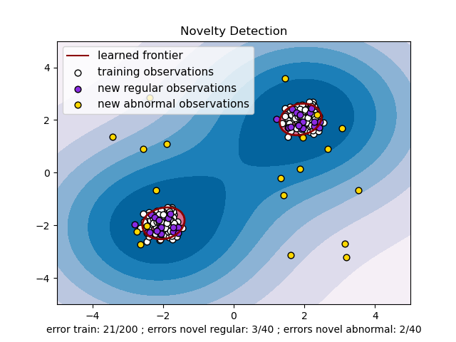
     最后的结果并不令人满意，为什么正常的会被判定成异常，如上图所示，确实有几个正常样本点有点离群，但是还有更多分布正常的点被隔离了出去。下面我们来对oneclassSVM进行分析，来找原因。

One-class SVM

首先，SVM是用一个超平面来区分类别一和类别二；而One-class SVM是用无数个超平面区分类别一和类别二三四...。也就是说用于区分本类和异类的边界是有无数超平面组成的。既然这样，这个方法中就应该有参数来调节超平面的选取，使它通融一下，放几个人进来（扩大边界）。

Parameters:

• kernel 根据经验判断数据可能是那种分布。‘linear’：线性；‘rbf’：高斯分布，默认的；等等
• nu 似乎使我们要找的参数，表示训练误差分数（0， 1]。就不能是0吗 (｀へ´)
• degree 当核函数是‘poly’多项式的时候有用，表示阶次。
• gamma 相关系数，默认1/n_features
• coef0 不懂
• tol 决定收敛的程度
• shrinking 不懂
• cache_size 没用，不管
• verbose 过程是否显示，默认不显示
• max_iter 最大迭代次数，默认-1，不限制
• random_state 加噪声

拨开云雾见天日，守得云开见月明！

     原来上面代码中 clf = svm.OneClassSVM(nu=0.1, kernel="rbf", gamma=0.1)中nu=0.1表示训练集里有10%的叛徒，我们可以把nu尽量调小，但不能是0，这样error train就变小了，但是errors novel abnormal可能会变大。可以交叉验证找一个平衡点。

PS：这里说一下我写这篇文章的目的。最近有一个需求，有n个数据集，每个数据集中有m个数据，每个数据集中的数据都服从高斯分布。但是，有些数据集（k个，k<n）中有异常点，不知道有多少个，我想把这些异常点找出来。约束条件是，不能把正常的判定为异常，尽量能找出所有异常。找一下sklearn里的工具，One-class SVM受参数nu的限制，我不知道对每个数据集把nu设为多少合适，果然还是不行。

异常点检测（Outlier Detection）

     异常点监测和奇异值检测有着相同的目的，都是为了把大部分数据聚集的簇与少量的噪声样本点分开。不同的是，对于异常点监测来说，我们没有一个干净的训练集（训练集中也有噪声样本）。

Fitting an elliptic envelope

     一个一般的思路是，假设常规数据隐含这一个已知的概率分布。基于这个假设，我们尝试确定数据的形状（边界），也可以将远离边界的样本点定义为异常点。SKlearn提供了一个covariance.EllipticEnvelope类，它可以根据数据做一个鲁棒的协方差估计，然后学习到一个包围中心样本点并忽视离群点的椭圆。 鲁棒的意思是足够稳定，即每次通过EllipticEnvelope对相同数据做出的协方差估计基本相同。

     举个例子，假设合群数据都是高斯分布的，那么EllipticEnvelope会鲁棒的估计合群数据的位置和协方差，而不会受到离群数据的影响。从该估计得到的马氏距离用于得出偏离度度量。例子如下：

import numpy as np
import matplotlib.pyplot as plt

from sklearn.covariance import EmpiricalCovariance, MinCovDet

n_samples = 125  # 125个训练集

n_outliers = 25  # 25个异常点

n_features = 2  # 2维的，为了方便在平面图上展示

# generate data
gen_cov = np.eye(n_features)  # 创建一个2*2的单位矩阵

gen_cov[0, 0] = 2.  # 矩阵的第一个元素改成2

# 随机数矩阵与上面的2*2矩阵点乘，就是为了把分布搞得像个椭圆

X = np.dot(np.random.randn(n_samples, n_features), gen_cov)

# add some outliers
outliers_cov = np.eye(n_features)

outliers_cov[np.arange(1, n_features), np.arange(1, n_features)] = 7.

X[-n_outliers:] = np.dot(np.random.randn(n_outliers, n_features), outliers_cov)  # 125个训练集中有25个被诱反

# fit a Minimum Covariance Determinant (MCD) robust estimator to data
robust_cov = MinCovDet().fit(X)  # 最小协方差确定

# compare estimators learnt from the full data set with true parameters

emp_cov = EmpiricalCovariance().fit(X)  # 最大协方差

fig  = plt .figure()
plt .subplots_adjust(hspace =-. 1, wspace =. 4, top =. 95, bottom =. 05)  # 设置坐标系（子图）之间的间距

# Show data set
subfig1  = plt .subplot( 3,  1,  1)
inlier_plot  = subfig1 .scatter(X[:,  0], X[:,  1],
                              color = 'black', label = 'inliers')
outlier_plot  = subfig1 .scatter(X[:,  0][ -n_outliers:], X[:,  1][ -n_outliers:],
                               color = 'red', label = 'outliers')
subfig1 .set_xlim(subfig1 .get_xlim()[ 0],  11.)  # [-5, 11]
subfig1 .set_title( "Mahalanobis distances of a contaminated data set:")

# Show contours of the distance functions

# np.linspace(-5, 11, 100)表示从-5到11的100个平均采样值

# np.meshgrid（）详解见下

xx, yy  =  np.meshgrid( np.linspace(plt .xlim()[ 0], plt .xlim()[ 1],  100),

                      np.linspace(plt .ylim()[ 0], plt .ylim()[ 1],  100))

# xx.ravel()把xx展开成一维

# np.c_使xx变成第一列，yy变成第二列

zz  =  np.c_[xx .ravel(), yy .ravel()]

# 然后根据马氏距离的平方做同心的椭圆

mahal_emp_cov  = emp_cov .mahalanobis(zz)
mahal_emp_cov  = mahal_emp_cov .reshape(xx .shape)
emp_cov_contour  = subfig1 .contour(xx, yy,  np.sqrt(mahal_emp_cov),
                                  cmap =plt .cm .PuBu_r,
                                  linestyles = 'dashed')

mahal_robust_cov  = robust_cov .mahalanobis(zz)
mahal_robust_cov  = mahal_robust_cov .reshape(xx .shape)
robust_contour  = subfig1 .contour(xx, yy,  np.sqrt(mahal_robust_cov),
                                 cmap =plt .cm .YlOrBr_r, linestyles = 'dotted')

subfig1 .legend([emp_cov_contour .collections[ 1], robust_contour .collections[ 1],
                inlier_plot, outlier_plot],
               [ 'MLE dist',  'robust dist',  'inliers',  'outliers'],
               loc = "upper right", borderaxespad = 0)
plt .xticks(())

plt .yticks(())

plt .show()

讲真，这个官方的代码太长了，实在看不懂。奈何想看的电影还没下完，硬着头皮上了╮(╯▽╰)╭

自己的理解都用注释的形式写在了上面。

np.meshgrid(x, y)

     返回两个相关向量（x，y）的相关矩阵。

1. Parameters：x，y是两个1维的向量，代表一个网格
2. Returns：返回矩阵X和Y，shape都是(len(y), len(x))，什么意思呢。

X表示所有交点的x坐标，Y表示所有交点的y坐标

mahalanobis(observations)

     计算给定观测样本点的马氏距离的平方

1. Parameters：观测点假定和之前训练用的数据集同分布
2. Returns：观测点的马氏距离的平方

这个椭圆边界法能不能解决我刚刚的问题呢？首先，输入是带有异常点的数据，且不需要给定有多少异常点掺在里面。但是，我该如何找到输入数据中的异常点呢。有没有输出阈值？？或者直接给出异常点的标签？？然而，我晕，突然发现sklearn Userguide的2.7.2.1下面给的例子不是elliptic envelope的，怪不得不对劲。查看sklearn.covariance.EllipticEnvelope的方法，果然有predict()。它的例子分析放在后面。

Isolation Forest

孤立森林是一个高效的异常点监测算法。SKLEARN提供了ensemble.IsolationForest模块。该模块在进行检测时，会随机选取一个特征，然后在所选特征的最大值和最小值随机选择一个分切面。该算法下整个训练集的训练就像一颗树一样，递归的划分。划分的次数等于根节点到叶子节点的路径距离d。所有随机树（为了增强鲁棒性，会随机选取很多树形成森林）的d的平均值，就是我们检测函数的最终结果。

那些路径d比较小的，都是因为距离主要的样本点分布中心比较远的。也就是说可以通过寻找最短路径的叶子节点来寻找异常点。它的例子也放在后面。

One-class SVM

严格来说，一分类的SVM并不是一个异常点监测算法，而是一个奇异点检测算法：它的训练集不能包含异常样本，否则的话，可能在训练时影响边界的选取。但是，对于高维空间中的样本数据集，如果它们做不出有关分布特点的假设，One-class SVM将是一大利器。

下面是对三种异常检测算法进行比较，EllipticEnvelope随着训练集变得unimodal效果下降，OneClassSVM会好一点，不受unimodel的影响，而IsolationForest在各种情况下都比较理想。

import  numpy  as  np
from  scipy  import stats
import  matplotlib.pyplot  as  plt
import  matplotlib.font_manager

from  sklearn  import svm
from  sklearn.covariance  import  EllipticEnvelope
from  sklearn.ensemble  import  IsolationForest

rng  = np .random .RandomState( 42)

# Example settings
n_samples  =  200
outliers_fraction  =  0.25
clusters_separation  = [ 0,  1,  2]

# define two outlier detection tools to be compared
classifiers  = {
     "One-Class SVM":  svm.OneClassSVM(nu = 0.95  * outliers_fraction  +  0.05,
                                     kernel = "rbf", gamma = 0.1),
     "Robust covariance":  EllipticEnvelope(contamination =outliers_fraction),
     "Isolation Forest":  IsolationForest(max_samples =n_samples,
                                        contamination =outliers_fraction,
                                        random_state =rng)}

# Compare given classifiers under given settings
xx, yy  =  np.meshgrid( np.linspace( - 7,  7,  500),  np.linspace( - 7,  7,  500))
n_inliers  =  int(( 1.  - outliers_fraction)  * n_samples)
n_outliers  =  int(outliers_fraction  * n_samples)
ground_truth  =  np.ones(n_samples, dtype = int)
ground_truth[ -n_outliers:]  =  - 1

# Fit the problem with varying cluster separation
for i, offset  in  enumerate(clusters_separation):
     np.random.seed( 42)
     # Data generation
    X1  =  0.3  *  np.random.randn(n_inliers  //  2,  2)  - offset
    X2  =  0.3  *  np.random.randn(n_inliers  //  2,  2)  + offset
    X  =  np.r_[X1, X2]
     # Add outliers
    X  =  np.r_[X, np .random .uniform(low =- 6, high = 6, size =(n_outliers,  2))]

     # Fit the model
    plt .figure(figsize =( 10.8,  3.6))
     for i, (clf_name, clf)  in  enumerate(classifiers .items()):
         # fit the data and tag outliers
        clf .fit(X)
        scores_pred  = clf .decision_function(X)
        threshold  =  stats.scoreatpercentile(scores_pred,
                                             100  * outliers_fraction)
        y_pred  = clf .predict(X)
        n_errors  = (y_pred  != ground_truth) .sum()
         # plot the levels lines and the points
        Z  = clf .decision_function( np.c_[xx .ravel(), yy .ravel()])
        Z  = Z .reshape(xx .shape)
        subplot  = plt .subplot( 1,  3, i  +  1)
        subplot .contourf(xx, yy, Z, levels = np.linspace(Z .min(), threshold,  7),
                         cmap =plt .cm .Blues_r)
        a  = subplot .contour(xx, yy, Z, levels =[threshold],
                            linewidths = 2, colors = 'red')
        subplot .contourf(xx, yy, Z, levels =[threshold, Z .max()],
                         colors = 'orange')
        b  = subplot .scatter(X[: -n_outliers,  0], X[: -n_outliers,  1], c = 'white')
        c  = subplot .scatter(X[ -n_outliers:,  0], X[ -n_outliers:,  1], c = 'black')
        subplot .axis( 'tight')
        subplot .legend(
            [a .collections[ 0], b, c],
            [ 'learned decision function',  'true inliers',  'true outliers'],
            prop =matplotlib .font_manager .FontProperties(size = 11),
            loc = 'lower right')
        subplot .set_title( " %d .  %s  (errors:  %d )"  % (i  +  1, clf_name, n_errors))
        subplot .set_xlim(( - 7,  7))
        subplot .set_ylim(( - 7,  7))
    plt .subplots_adjust( 0.04,  0.1,  0.96,  0.92,  0.1,  0.26)

plt .show()

在上面三种分类器的定义中，都需要给定outliers_fraction，也就是说都需要知道原始训练集中有多少异常点，所以都不符合我当前问题的需要。