Day 15 复习日——自选数据集

@浙大疏锦行

今日任务：

1. 尝试找到一个kaggle或者其他地方的结构化数据集，用之前的内容完成一个全新的项目。
2. 探索开源的数据网站

今天主要是将之前所学的内容进行回顾，自己选择一个数据集将机器学习的完整流程进行实践。首先简要回顾完整流程：

• 数据获取：明确研究的问题（回归 or 分类），确定标签和特征
• 数据查看：明确数据的基本信息
• 数据预处理：缺失值填充、异常值处理、数据类型转换（标签编码和独热编码）、连续特征处理（特征尺度统一，标准化与归一化）。若为分类问题，考虑不平衡数据的处理，使用过采样、权重设置和阈值调整等方法
• 描述性统计分析：数据初步可视化，探索特征分布、特征间的关系等
• 特征工程：删除不重要的特征和创造新的特征
• 模型训练与评估：划分数据集后，对比多模型进行训练，使用评估指标进行评估。选择其中效果好的模型进行超参数调整（贝叶斯优化，网格搜索）
• 对训练的结果进行可解释性分析（SHAP）

开源数据网站：

Kaggle：https://www.kaggle.com/datasets

UCI Machine Learning Repository： https://archive.ics.uci.edu/ml

阿里云天池：天池数据集_阿里系唯一对外开放数据分享平台-阿里云天池

和鲸社区：数据集 - Heywhale.com

除了上述所列，还有许多，比如政府开放数据、学术数据共享等等

选择Entrepreneurial Competency in University Students进行分析，地址为：https://www.kaggle.com/namanmanchanda/entrepreneurial-competency-in-university-students

数据总共219行，17列。下面是列的说明：

列名	含义
EducationSector	教育部门（8个类别）
IndividualProject	个人项目 Yes/No
Age	学生年龄 （17-26）
Gender	学生性别 Male/Female
City	是否在城市 Yes/No
Influenced	影响 Yes/No
Perseverance	毅力（1,2,3,4,5）
DesireToTakeInitiative	积极主动的愿望（1,2,3,4,5）
Competitiveness	竞争力（1,2,3,4,5）
SelfReliance	自力更生（1,2,3,4,5）
StrongNeedToAchieve	强烈的实现需求（1,2,3,4,5）
SelfConfidence	自信心（1,2,3,4,5）
GoodPhysicalHealth	良好的身体健康等级（1,2,3,4,5）
MentalDisorder	是否有精神障碍 Yes/No
KeyTraits	学生的主要特征（5个类别）
ReasonsForLack	缺乏的原因（各种各样）
y	学生是否成为企业家 0/1

导入库

import pandas as pd
import matplotlib.pyplot as plt
import seaborn as sns
from sklearn.model_selection import train_test_split
from sklearn.metrics import accuracy_score,precision_score,recall_score,f1_score
from sklearn.metrics import confusion_matrix,classification_report
import shap
import numpy as np

#绘图中中文显示问题
#绘图中负号显示问题

数据查看

data = pd.read_csv(r'university_students.csv')
data.info()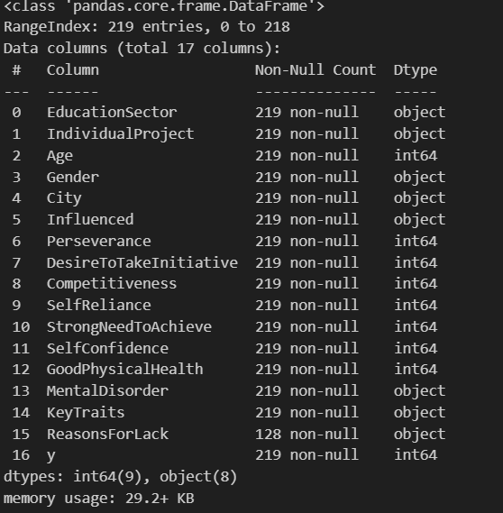

data.info()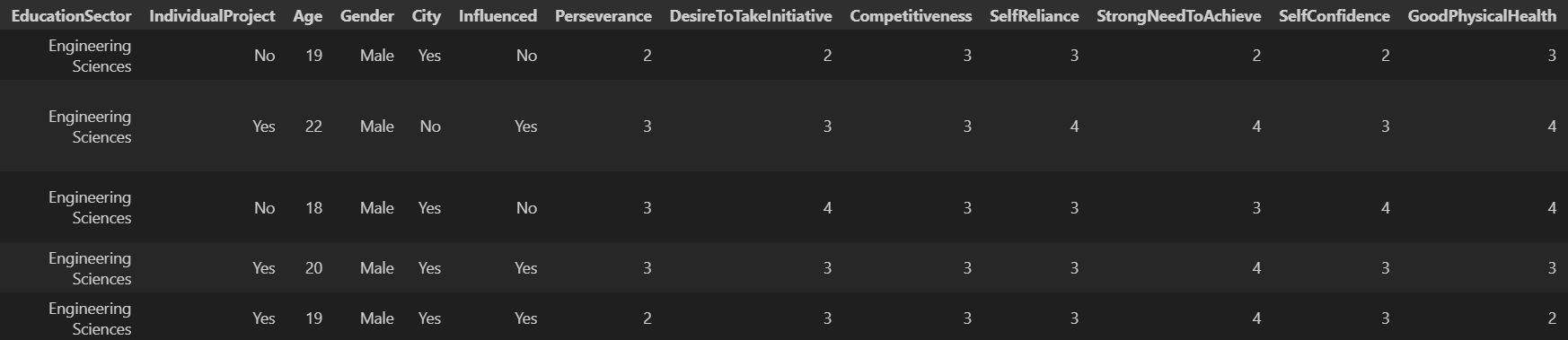

数据预处理

通过概览信息的查看，可以得到数据无缺失值。异常值先不考虑。对于16个特征中，有8个属于obejct类型，其中ReasonsForLack列的内容太杂，暂时删去。剩下的有4个列均为‘Yes/No’型和1个‘男/女’，采用标签编码映射；2个为多类别的无序特征，选择使用独热编码。

#离散特征和连续特征
#continous_features = data.select_dtypes(include=['float64','int64']).columns.tolist()
#discrete_features = data.select_dtypes(include=['object']).columns.tolist()
#编码
#1-标签编码,0-1映射
mapping_dict = {
	'IndividualProject':{
        'No':0,
        'Yes':1
	},
    'City':{
        'No':0,
        'Yes':1
	},
    'Influenced':{
        'No':0,
        'Yes':1
	},
    'MentalDisorder':{
        'No':0,
        'Yes':1
	},
    'Gender':{
        'Female':0,
        'Male':1
	}
}
for key,value in mapping_dict.items():
	data[key] = data[key].map(value)

data.rename(columns={'Gender': 'Male'}, inplace=True) # 重命名列,0-1映射

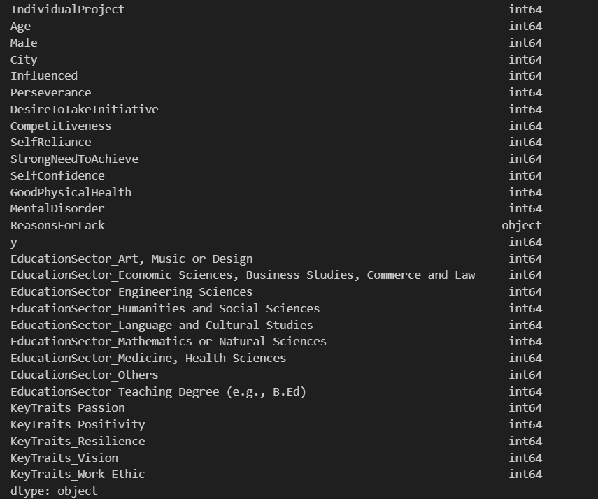
#2-独热编码
data = pd.get_dummies(data,columns=['EducationSector','KeyTraits'])
data_1 = pd.read_csv(r'university_students.csv')
new_features = []
for i in data:
    if i not in data_1:
        new_features.append(i)
for j in new_features:
    data[j] = data[j].astype(int)
data.dtypes

查看标签的分布情况，两种类别比例在1.41:1，不平衡问题较轻

data['y'].value_counts()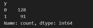

不进行过采样处理，但简单回顾处理方法：

#不平衡数据的处理,对训练集进行处理
#导入库
from sklearn.over_sampling import SMOTE
#SMOTE过采样
smote = SMOTE(random_state=42)
X_smote,y_smote = smote.fit_resample(X_train,y_train)

描述性分析

之前学习的图形主要有直方图、箱形图、小提琴图、计数图和热图。此外还知道了绘制子图的方法。

#描述性统计
continuous_features = data.select_dtypes(include=['int64']).columns.to_list()
#设置画布
fig,axes = plt.subplots(3,3,figsize=(12,12))
axes = axes.flatten()

for index,value in enumerate(continuous_features[:9]): #查看前9个
	sns.countplot(data=data,x=value,ax=axes[index])
	axes[index].set_xlabel(value)
	axes[index].set_title(f'The Countplot of {value}')
plt.tight_layout()
plt.show()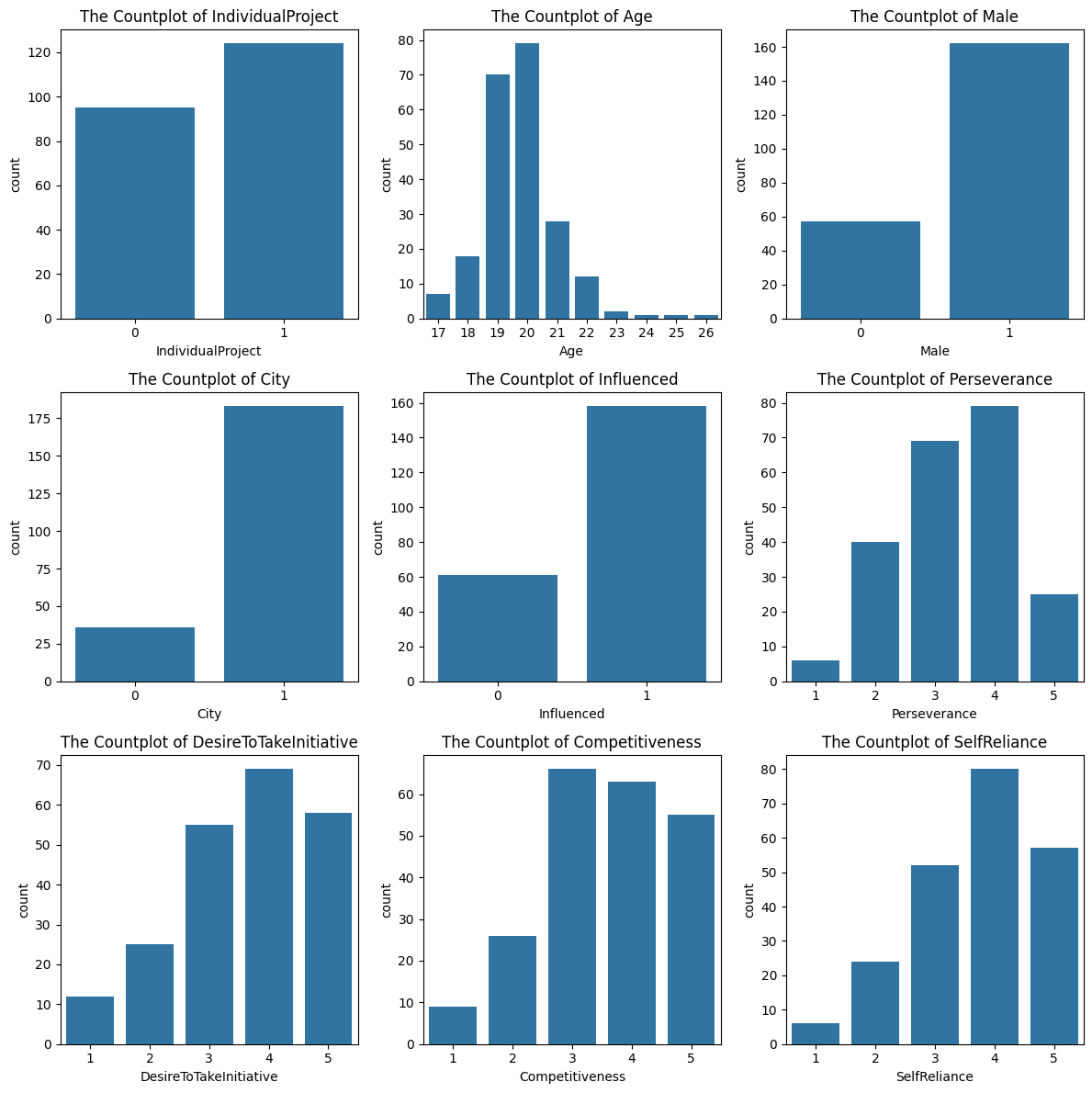

建模与训练

#设置标签和特征
X = data.drop(['y','ReasonsForLack'],axis=1) #由于ReasonsForLack列的东西太杂，选择删去
y = data['y']
#数据集的划分
X_train,X_test,y_train,y_test = train_test_split(X,y,train_size=0.8,random_state=42)

#确定少数类
counts = np.bincount(y)
minority_class = np.argmin(counts)

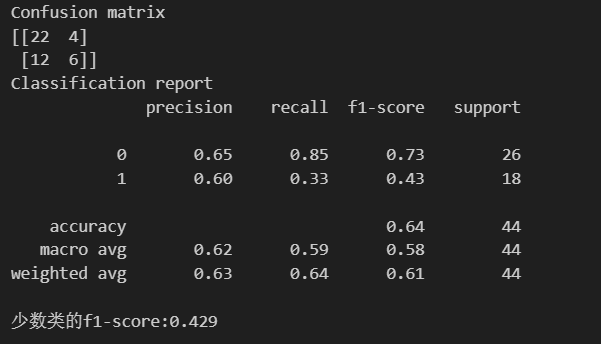
随机森林

#导入模型训练
from sklearn.ensemble import RandomForestClassifier

#核心三行代码
rf_model = RandomForestClassifier(random_state=42) #实例化
rf_model.fit(X_train,y_train) #训练，此处未考虑过采样
rf_pred = rf_model.predict(X_test) #预测

#评估指标
print('Confusion matrix')
print('{}'.format(confusion_matrix(y_test,rf_pred)))
print('Classification report')
print('{}'.format(classification_report(y_test,rf_pred)))

#查看少数类的f1-score
print('少数类的f1-score:{:.3f}'.format(f1_score(y_test,rf_pred,pos_label=minority_class)))

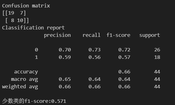
XGBoost

#导入模型训练
from xgboost import XGBClassifier

#核心三行代码
xgb_model = XGBClassifier(random_state=42) #实例化
xgb_model.fit(X_train,y_train) #训练，此处未考虑过采样
xgb_pred = xgb_model.predict(X_test) #预测

#评估指标
print('Confusion matrix')
print('{}'.format(confusion_matrix(y_test,xgb_pred)))
print('Classification report')
print('{}'.format(classification_report(y_test,xgb_pred)))

#查看少数类的f1-score
print('少数类的f1-score:{:.3f}'.format(f1_score(y_test,xgb_pred,pos_label=minority_class)))

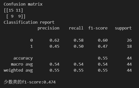
KNN

#导入模型训练
from sklearn.neighbors import KNeighborsClassifier

#核心三行代码
knn_model = KNeighborsClassifier() #实例化
knn_model.fit(X_train,y_train) #训练，此处未考虑过采样
knn_pred = knn_model.predict(X_test) #预测

#评估指标
print('Confusion matrix')
print('{}'.format(confusion_matrix(y_test,knn_pred)))
print('Classification report')
print('{}'.format(classification_report(y_test,knn_pred)))

#查看少数类的f1-score
print('少数类的f1-score:{:.3f}'.format(f1_score(y_test,knn_pred,pos_label=minority_class)))

超参数调整

根据F1-Score作为评估标准，选择XGBoost进行超参数调参（贝叶斯优化）

#导入库
from skopt import BayesSearchCV
from skopt.space import Integer
import time

start_time = time.time()
#设置参数空间
search_spaces = {
    'n_estimators':Integer(50,200),
    'max_depth':Integer(10,30),
    'min_samples_split':Integer(2,10),
    "min_sampls_leaf":Integer(1,4)
}
#实例化
bayes_search = BayesSearchCV(
    estimator=XGBClassifier(random_state=42),
    search_spaces=search_spaces,
    n_iter=25,
    cv=5,
    n_jobs=-1,
    scoring='f1' #使用f1分数评估
)
#训练
bayes_search.fit(X_train,y_train)
end_time = time.time()
print('调参所需时间：{:.4f}s'.format(end_time-start_time))

#获取最佳模型、参数，训练
best_xgb_model = bayes_search.best_estimator_
best_xgb_pred = best_xgb_model.predict(X_test)

#评估指标
print('Confusion matrix')
print('{}'.format(confusion_matrix(y_test,best_xgb_pred)))
print('Classification report')
print('{}'.format(classification_report(y_test,best_xgb_pred)))

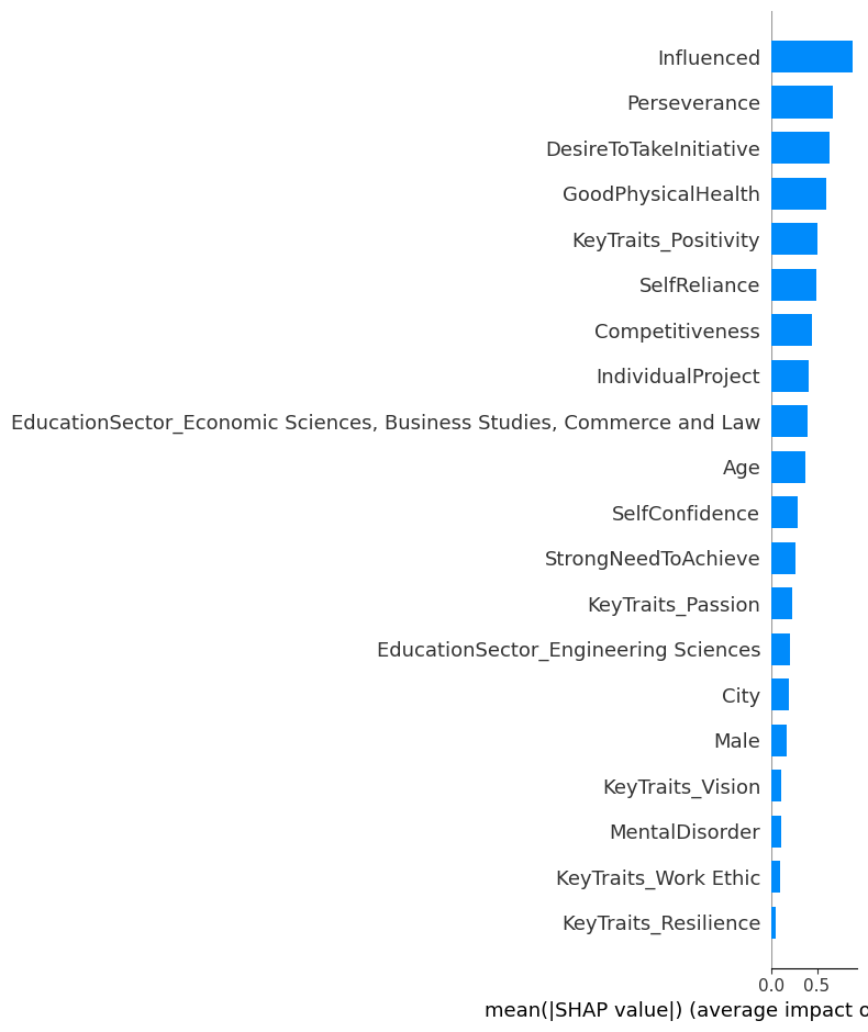
可解释性分析

#初始化解释器
explainer = shap.TreeExplainer(xgb_model)

#计算shap值
shap_values = explainer.shap_values(X_test)

#查看shap_value数组的尺寸(44,27),表示每个特征对预测为正类的对数几率的贡献

#绘制图形，查看特征重要性
shap.summary_plot(shap_values, X_test, plot_type='bar',feature_names=X_test.columns.tolist())

通过今日的练习，将之前所学的内容，基本都有回顾和操作。但是对于这个数据的分析是十分粗糙的，在很多地方需要优化，来挖掘数据的价值。