


 本文详细介绍如何使用Python从零开始构建神经网络,涵盖激活函数、正则化、优化算法及梯度检验等内容,通过实际代码实现加深理解。
目录
一篇文章让你实现PYTHON手写神经网络+优化+正则化+梯度检验
主函数
import numpy as np
import matplotlib.pyplot as plt
import math
import my
plt.rcParams['figure.figsize'] = (7.0, 4.0) # 图片像素
plt.rcParams['image.interpolation'] = 'nearest' # 设置 interpolation style
plt.rcParams['image.cmap'] = 'gray' # 设置 颜色 style
def model(X, Y,activation, layers_dims, learning_rate=0.03, num_iterations=3000, print_cost=True, alpha = 0, keep_prob = 1, initialzation="zero", is_plot=True, mini_batch_size=1, grad_option='Adam', beta1 = 0.9, beta2 = 0.999):
costs = []
m = X.shape[1]
S = {}
v = {}
t = 0 # 用于让开始的数值平滑
for i in range(1, len(layers_dims)):
if grad_option == 'RMSprop':
beta1 = 0
v['dW' + str(i)] = np.ones((layers_dims[i], 1))
v['db' + str(i)] = np.ones((layers_dims[i], 1))
else:
v['dW' + str(i)] = np.zeros((layers_dims[i], 1))
v['db' + str(i)] = np.zeros((layers_dims[i], 1))
if grad_option == 'Momentum':
beta2 = 0
S['dW' + str(i)] = np.ones((layers_dims[i], 1))
S['db' + str(i)] = np.ones((layers_dims[i], 1))
else:
S['dW'+str(i)] = np.zeros((layers_dims[i], 1))
S['db' + str(i)] = np.zeros((layers_dims[i], 1))
# 选择初始参数类型
parameters = my.initialize_parameters(layers_dims, initialzation)
for i in range(0, num_iterations):
t = t+1
# 打乱训练数据的顺序
permutation = list(np.random.permutation(m))
shuffled_X = X[:, permutation]
shuffled_Y = Y[:, permutation].reshape((1, m))
# 第二步,分割
num_complete_minibatches = math.floor(m / mini_batch_size)
for k in range(num_complete_minibatches):
if k == num_complete_minibatches - 1:
temp_X = shuffled_X[:, k * mini_batch_size:]
temp_Y = shuffled_Y[:, k * mini_batch_size:]
else:
temp_X = shuffled_X[:, k * mini_batch_size:(k+1)*mini_batch_size]
temp_Y = shuffled_Y[:, k * mini_batch_size:(k+1)*mini_batch_size]
pred, for_res = my.forward_propagation(temp_X, parameters, activation, keep_prob) # 前向传播
cost = my.compute_loss_with_regularization(pred, temp_Y, parameters, alpha) # 计算损失,可以没有
grads = my.backward_propagation(temp_X, temp_Y, for_res, alpha, keep_prob) # 反向传播
if i == 1000:
print(my.gradient_check(X=temp_X, Y=temp_Y, grads=grads, parameters=parameters, activation=activation, alpha=alpha, epsilon=1e-7))
parameters = my.update_parameters(parameters, grads, learning_rate, t=t, v=v, S=S, beta1=beta1, beta2=beta2, grad_option=grad_option) # 更新参数
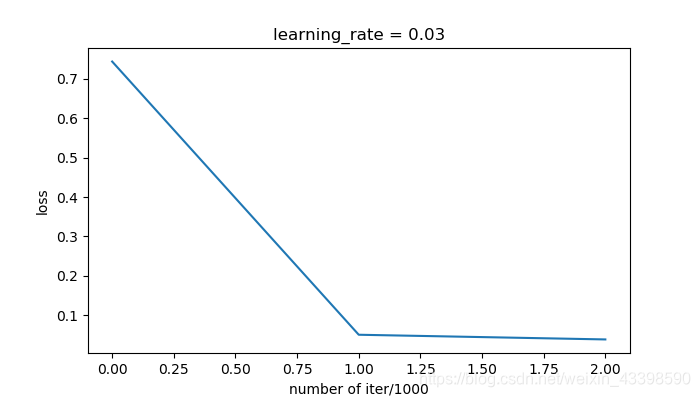
if i % 1000 == 0:
costs.append(cost)
if print_cost:
print("第" + str(i) + "次迭代,成本值为:" + str(cost))
if is_plot:
plt.plot(costs)
plt.ylabel('loss')
plt.xlabel('number of iter/1000')
plt.title("learning_rate = " + str(learning_rate))
plt.show()
return parameters
train_X, train_Y, test_X, test_Y = my.load_dataset(is_plot=True)
activation = [0, 0, 1]
layers_dims = [train_X.shape[0], 20, 3, 1]
parameters = model(train_X, train_Y, activation=activation, layers_dims=layers_dims, alpha=0.01, mini_batch_size=math.floor(train_X.shape[1]/10), keep_prob=1, grad_option='Adam', is_plot=True, initialzation="random")
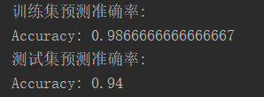
print("训练集预测准确率:")
predictions_train = my.predict(train_X, train_Y, parameters, activation)
print("测试集预测准确率:")
predictions_test = my.predict(test_X, test_Y, parameters, activation)
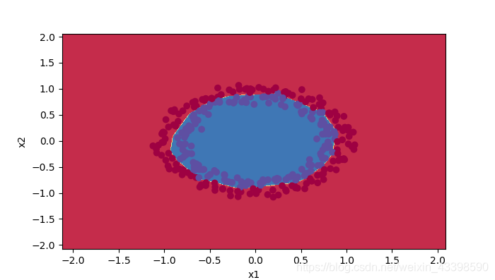
my.plot_decision_boundary(lambda x: my.predict_dec(parameters, x.T, activation), train_X, train_Y)
功能简介
激活函数支持sigmoid和rule两种,其中0代表rule,1代表sigmoid。
加速训练的方式有Momentum,RMSprop和Adam,以及minibatch方法。
参数初始化方式有0初始化,随机初始化和抑梯度异常初始化。
正则化方式有常用的L2正则化以及dropout。
my.py
需要的包
import numpy as np
import matplotlib.pyplot as plt
import sklearn
import sklearn.datasets
读取数据
我们的数据从sklearn的库中随机生成。
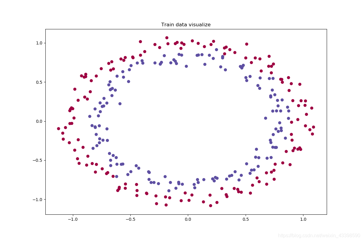
def load_dataset(is_plot=True):
    np.random.seed(1)  # 设置随机数种子
    train_X, train_Y = sklearn.datasets.make_circles(n_samples=300, noise=.05)  # 随机生成数据
    np.random.seed(2)  # 设置随机数种子
    test_X, test_Y = sklearn.datasets.make_circles(n_samples=100, noise=.05)
    if(is_plot):
        fig, ax = plt.subplots(nrows=1, ncols=1, figsize=(12, 8))
        ax.scatter(train_X[:, 0], train_X[:, 1], c=train_Y, s=40, cmap=plt.cm.Spectral)  # 给不同数字不同颜色
        ax.set_title('Train data visualize')
        plt.show()
    return train_X.T, train_Y.reshape((1, train_Y.shape[0])), test_X.T, test_Y.reshape((1, test_Y.shape[0]))
初始化参数
如果用0初始化会导致每层W,b的值都相同,所以一般不用。
def initialize_parameters(layers_dims, option):
    parameters = {}
    L = len(layers_dims)  # 网络层数
    for l in range(1, L):
        if option == 'zero':
            parameters["W" + str(l)] = np.zeros((layers_dims[l], layers_dims[l - 1]))
        elif option == 'random':
            parameters['W' + str(l)] = np.random.randn(layers_dims[l], layers_dims[l - 1])
        else:
            np.random.seed(3)
            parameters['W' + str(l)] = np.random.randn(layers_dims[l], layers_dims[l - 1]) * np.sqrt(2 / layers_dims[l - 1])
        parameters["b" + str(l)] = np.zeros((layers_dims[l], 1))
        # 使用断言确保我的数据格式是正确的
        assert (parameters["W" + str(l)].shape == (layers_dims[l], layers_dims[l - 1]))
        assert (parameters["b" + str(l)].shape == (layers_dims[l], 1))
    return parameters
激活函数
def sigmoid(x):
    s = 1/(1+np.exp(-x))
    return s


def relu(x):
    s = np.maximum(0, x)
    return s
前向传播与反向传播
def forward_propagation(X, parameters, activation, keep_prob = 1):
    for_res = {}
    for_res['a' + str(0)] = X
    for_res['activation'] = activation
    L = len(parameters) // 2
    for i in range(1, L + 1):
        for_res['b' + str(i)] = parameters['b' + str(i)]
        for_res['W' + str(i)] = parameters['W' + str(i)]
        for_res['z' + str(i)] = np.dot(parameters['W' + str(i)], for_res['a' + str(i - 1)]) + parameters['b' + str(i)]
        if activation[i - 1] == 0:
            for_res['a' + str(i)] = relu(for_res['z' + str(i)])
        else:
            for_res['a' + str(i)] = sigmoid(for_res['z' + str(i)])
        if i != L:
            for_res['d' + str(i)] = np.random.rand(for_res['a' + str(i)].shape[0], for_res['a' + str(i)].shape[1])
            for_res['d' + str(i)] = for_res['d' + str(i)] <= keep_prob  # 进行dropout操作,第一层和最后一层不需要。
            for_res['a' + str(i)] = np.multiply(for_res['a' + str(i)], for_res['d' + str(i)])
    return for_res['a' + str(L)], for_res
def backward_propagation(X, Y, for_res, alpha, keep_prob):
    grads = {}
    m = X.shape[1]
    L = len(for_res) // 5
    grads['dz' + str(L)] = 1. / m * (for_res['a'+str(L)] - Y)
    for i in range(L, 0, -1):
        if i != L:
            grads['da' + str(i)] = np.dot(for_res['W' + str(i + 1)].T, grads['dz' + str(i + 1)])  # 注意有转置
            grads['da' + str(i)] = np.multiply(grads['da' + str(i)], for_res['d' + str(i)]) / keep_prob
            if for_res['activation'][i - 1] == 0:
                grads['dz' + str(i)] = np.multiply(grads['da' + str(i)], np.int64(for_res['a' + str(i)] > 0))  # relu函数求导
            else:
                grads['dz' + str(i)] = np.multiply(grads['da' + str(i)], np.multiply(for_res['a' + str(i)], 1 - for_res['a' + str(i)]))
        grads['dW' + str(i)] = np.dot(grads['dz' + str(i)], for_res['a' + str(i - 1)].T) + alpha * for_res['W' + str(i)] / m  # 前一项是梯度,后一项是正则化项,注意有转置
        grads['db' + str(i)] = np.sum(grads['dz' + str(i)], axis=1, keepdims=True)  # 计算back_res['db' + str(i)]的梯度,按行求和
    return grads
损失值计算
def compute_loss(pred, Y):
    return np.nansum(np.multiply(-np.log(pred), Y) + np.multiply(-np.log(1 - pred), 1 - Y)) * 1. / Y.shape[1]


def compute_loss_with_regularization(pred, Y, parameters, alpha):
    L = len(parameters) // 2
    n = 0
    for i in range(1, L + 1):
        n += np.sum(np.square(parameters['W' + str(i)]))
    return compute_loss(pred, Y) + n * alpha / (2 * Y.shape[1])
参数更新
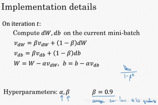
这三种方法都利用了指数加权平均的思路,来加快训练速度。
Momentum
为了避免训练一开始时,之前没有数据导致的前次训练梯度偏小的情况,我们让我们的
v
=
v
1
−
β
t
v=\frac{v}{1-\beta^t}
v=1−βtv,这样在一开始
v
v
v的值会变大,随着
t
t
t的增大,分母趋于1。
RMSprop
你执行梯度下降,虽然横轴方向正在推进,但纵轴方向会有大幅度摆动,为了减少纵轴方法的摆动,我们引入了方差。同样,为了避免训练一开始时,之前没有数据导致的前次训练梯度偏小的情况,我们让我们的 v = v 1 − β t v=\frac{v}{1-\beta^t} v=1−βtv,这样在一开始 v v v的值会变大,随着 t t t的增大,分母趋于1。

Adam
这个就是把上面两个方法叠加在一起。
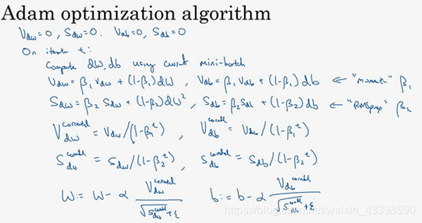
def update_parameters(parameters, grads, learning_rate, t, v, S, beta1, beta2, grad_option):
    epsilon = 1e-8
    L = len(parameters) // 2  # 向下取整
    for i in range(1, L + 1):
        if grad_option == 'Adam' or grad_option == 'Momentum':
            v['dW' + str(i)] = beta1 * v['dW' + str(i)] + (1 - beta1) * grads["dW" + str(i)]
            v['db' + str(i)] = beta1 * v['db' + str(i)] + (1 - beta1) * grads["db" + str(i)]
        else:
            v['dW' + str(i)] = grads["dW" + str(i)]
            v['db' + str(i)] = grads["db" + str(i)]
        if grad_option == 'Adam' or grad_option == 'RMSprop':
            S['dW' + str(i)] = beta2 * S['dW' + str(i)] + (1 - beta2) * np.square(grads["dW" + str(i)])
            S['db' + str(i)] = beta2 * S['db' + str(i)] + (1 - beta2) * np.square(grads["db" + str(i)])
        parameters["W" + str(i)] = parameters["W" + str(i)] - learning_rate * v['dW' + str(i)] / ((np.sqrt(S['dW' + str(i)]) + epsilon) / (1 - np.power(beta2, t)) * (1 - np.power(beta1, t)))
        parameters["b" + str(i)] = parameters["b" + str(i)] - learning_rate * v['db' + str(i)] / ((np.sqrt(S['db' + str(i)]) + epsilon) / (1 - np.power(beta2, t)) * (1 - np.power(beta1, t)))
    return parameters
梯度检验
我们的梯度检验就相当于对每一个参数在给定情况下的导数值求一个近似,来比较其与我们求得的梯度的差距。
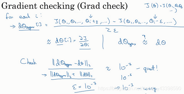
注意:使用dropout时不能进行梯度检,因为每次迭代过程中,dropout会随机消除隐藏层单元的不同子集,难以计算dropout在梯度下降上的代价函数
J
J
J。
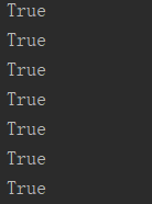
可以看到我们的梯度检验全部通过。
def gradient_check(X, Y, grads, parameters, alpha, activation, epsilon=1e-7):
    L = len(parameters) // 2
    check = True
    for i in range(1, L + 1):
        L1 = np.zeros(parameters['W' + str(i)].shape)
        L2 = np.zeros(parameters['W' + str(i)].shape)
        for j in range(parameters['W' + str(i)].shape[0]):
            for k in range(parameters['W' + str(i)].shape[1]):
                parameters['W' + str(i)][j, k] -= epsilon
                pred, for_res = forward_propagation(X, parameters, activation, keep_prob=1)
                L1[j, k] = compute_loss_with_regularization(pred, Y, parameters, alpha)
                parameters['W' + str(i)][j, k] += 2 * epsilon
                pred, for_res = forward_propagation(X, parameters, activation, keep_prob=1)
                L2[j, k] = compute_loss_with_regularization(pred, Y, parameters, alpha)
                parameters['W' + str(i)][j, k] -= epsilon
        grads_approx = (L2 - L1) / (2 * epsilon)

        val_1 = np.linalg.norm(grads_approx - grads['dW' + str(i)])
        val_2 = np.linalg.norm(grads_approx) + np.linalg.norm(grads['dW' + str(i)])
        if(val_1 / val_2 > 1e-7):
            print('w' + str(i))
            print(val_1 / val_2)
            check = False
        L1 = np.zeros(parameters['b' + str(i)].shape)
        L2 = np.zeros(parameters['b' + str(i)].shape)
        for j in range(parameters['b' + str(i)].shape[0]):
            parameters['b' + str(i)][j] -= epsilon
            pred, for_res = forward_propagation(X, parameters, activation, keep_prob=1)
            L1[j] = compute_loss_with_regularization(pred, Y, parameters, alpha)
            parameters['b' + str(i)][j] += 2 * epsilon
            pred, for_res = forward_propagation(X, parameters, activation, keep_prob=1)
            L2[j] = compute_loss_with_regularization(pred, Y, parameters, alpha)
            parameters['b' + str(i)][j] -= epsilon
        grads_approx = (L2 - L1) / (2 * epsilon)

        val_1 = np.linalg.norm(grads_approx - grads['db' + str(i)])
        val_2 = np.linalg.norm(grads_approx) + np.linalg.norm(grads['db' + str(i)])
        if (val_1 / val_2 > 1e-7):
            print('b' + str(i))
            print(val_1 / val_2)
            check = False
    return check
预测和结果图绘制
def predict(X, y, parameters, activation):
    a3, for_res = forward_propagation(X, parameters, activation)
    p = np.int64(a3 > 0.5)
    print("Accuracy: " + str(np.mean((p[0, :] == y[0, :]))))
    return p
def predict_dec(parameters, X, activation):
    a3, for_res = forward_propagation(X, parameters, activation)
    predictions = (a3 > 0.5)
    return predictions
def plot_decision_boundary(model, X, y):
    x_min, x_max = X[0, :].min() - 1, X[0, :].max() + 1
    y_min, y_max = X[1, :].min() - 1, X[1, :].max() + 1
    h = 0.01
    xx, yy = np.meshgrid(np.arange(x_min, x_max, h), np.arange(y_min, y_max, h))  # 返回坐标网格矩阵
    Z = model(np.c_[xx.ravel(), yy.ravel()])
    Z = Z.reshape(xx.shape)
    plt.contourf(xx, yy, Z, cmap=plt.cm.Spectral)
    plt.ylabel('x2')
    plt.xlabel('x1')
    plt.scatter(X[0, :], X[1, :], c=np.squeeze(y), cmap=plt.cm.Spectral)
    plt.show()
附录(完整代码)
主文件
import numpy as np
import matplotlib.pyplot as plt
import math
import my

plt.rcParams['figure.figsize'] = (7.0, 4.0)  # 图片像素
plt.rcParams['image.interpolation'] = 'nearest'  # 设置 interpolation style
plt.rcParams['image.cmap'] = 'gray'  # 设置 颜色 style

def model(X, Y,activation, layers_dims, learning_rate=0.03, num_iterations=3000, print_cost=True, alpha = 0, keep_prob = 1, initialzation="zero", is_plot=True, mini_batch_size=1, grad_option='Adam', beta1 = 0.9, beta2 = 0.999):
    costs = []
    m = X.shape[1]
    S = {}
    v = {}
    t = 0  # 用于让开始的数值平滑
    for i in range(1, len(layers_dims)):
        if grad_option == 'RMSprop':
            beta1 = 0
            v['dW' + str(i)] = np.ones((layers_dims[i], 1))
            v['db' + str(i)] = np.ones((layers_dims[i], 1))
        else:
            v['dW' + str(i)] = np.zeros((layers_dims[i], 1))
            v['db' + str(i)] = np.zeros((layers_dims[i], 1))
        if grad_option == 'Momentum':
            beta2 = 0
            S['dW' + str(i)] = np.ones((layers_dims[i], 1))
            S['db' + str(i)] = np.ones((layers_dims[i], 1))
        else:
            S['dW'+str(i)] = np.zeros((layers_dims[i], 1))
            S['db' + str(i)] = np.zeros((layers_dims[i], 1))
    # 选择初始参数类型
    parameters = my.initialize_parameters(layers_dims, initialzation)
    for i in range(0, num_iterations):
        t = t+1
        # 打乱训练数据的顺序
        permutation = list(np.random.permutation(m))
        shuffled_X = X[:, permutation]
        shuffled_Y = Y[:, permutation].reshape((1, m))
        # 第二步,分割
        num_complete_minibatches = math.floor(m / mini_batch_size)
        for k in range(num_complete_minibatches):
            if k == num_complete_minibatches - 1:
                temp_X = shuffled_X[:, k * mini_batch_size:]
                temp_Y = shuffled_Y[:, k * mini_batch_size:]
            else:
                temp_X = shuffled_X[:, k * mini_batch_size:(k+1)*mini_batch_size]
                temp_Y = shuffled_Y[:, k * mini_batch_size:(k+1)*mini_batch_size]
            pred, for_res = my.forward_propagation(temp_X, parameters, activation, keep_prob)  # 前向传播
            cost = my.compute_loss_with_regularization(pred, temp_Y, parameters, alpha)  # 计算损失,可以没有
            grads = my.backward_propagation(temp_X, temp_Y, for_res, alpha, keep_prob)  # 反向传播
            if i == 1000:
                print(my.gradient_check(X=temp_X, Y=temp_Y, grads=grads, parameters=parameters, activation=activation, alpha=alpha, epsilon=1e-7))
            parameters = my.update_parameters(parameters, grads, learning_rate, t=t, v=v, S=S, beta1=beta1, beta2=beta2, grad_option=grad_option)  # 更新参数
        if i % 1000 == 0:
            costs.append(cost)
            if print_cost:
                print("第" + str(i) + "次迭代,成本值为:" + str(cost))
    if is_plot:
        plt.plot(costs)
        plt.ylabel('loss')
        plt.xlabel('number of iter/1000')
        plt.title("learning_rate = " + str(learning_rate))
        plt.show()
    return parameters


train_X, train_Y, test_X, test_Y = my.load_dataset(is_plot=True)
activation = [0, 0, 1]
layers_dims = [train_X.shape[0], 20, 3, 1]
parameters = model(train_X, train_Y, activation=activation, layers_dims=layers_dims, alpha=0.01, mini_batch_size=math.floor(train_X.shape[1]/10), keep_prob=1, grad_option='Adam', is_plot=True, initialzation="random")
print("训练集预测准确率:")
predictions_train = my.predict(train_X, train_Y, parameters, activation)
print("测试集预测准确率:")
predictions_test = my.predict(test_X, test_Y, parameters, activation)
my.plot_decision_boundary(lambda x: my.predict_dec(parameters, x.T, activation), train_X, train_Y)
my.py
import numpy as np
import matplotlib.pyplot as plt
import sklearn
import sklearn.datasets


def sigmoid(x):
    s = 1/(1+np.exp(-x))
    return s


def relu(x):
    s = np.maximum(0, x)
    return s


def compute_loss(pred, Y):
    return np.nansum(np.multiply(-np.log(pred), Y) + np.multiply(-np.log(1 - pred), 1 - Y)) * 1. / Y.shape[1]


def compute_loss_with_regularization(pred, Y, parameters, alpha):
    L = len(parameters) // 2
    n = 0
    for i in range(1, L + 1):
        n += np.sum(np.square(parameters['W' + str(i)]))
    return compute_loss(pred, Y) + n * alpha / (2 * Y.shape[1])


def gradient_check(X, Y, grads, parameters, alpha, activation, epsilon=1e-7):
    L = len(parameters) // 2
    check = True
    for i in range(1, L + 1):
        L1 = np.zeros(parameters['W' + str(i)].shape)
        L2 = np.zeros(parameters['W' + str(i)].shape)
        for j in range(parameters['W' + str(i)].shape[0]):
            for k in range(parameters['W' + str(i)].shape[1]):
                parameters['W' + str(i)][j, k] -= epsilon
                pred, for_res = forward_propagation(X, parameters, activation, keep_prob=1)
                L1[j, k] = compute_loss_with_regularization(pred, Y, parameters, alpha)
                parameters['W' + str(i)][j, k] += 2 * epsilon
                pred, for_res = forward_propagation(X, parameters, activation, keep_prob=1)
                L2[j, k] = compute_loss_with_regularization(pred, Y, parameters, alpha)
                parameters['W' + str(i)][j, k] -= epsilon
        grads_approx = (L2 - L1) / (2 * epsilon)

        val_1 = np.linalg.norm(grads_approx - grads['dW' + str(i)])
        val_2 = np.linalg.norm(grads_approx) + np.linalg.norm(grads['dW' + str(i)])
        if(val_1 / val_2 > 1e-7):
            print('w' + str(i))
            print(val_1 / val_2)
            check = False
        L1 = np.zeros(parameters['b' + str(i)].shape)
        L2 = np.zeros(parameters['b' + str(i)].shape)
        for j in range(parameters['b' + str(i)].shape[0]):
            parameters['b' + str(i)][j] -= epsilon
            pred, for_res = forward_propagation(X, parameters, activation, keep_prob=1)
            L1[j] = compute_loss_with_regularization(pred, Y, parameters, alpha)
            parameters['b' + str(i)][j] += 2 * epsilon
            pred, for_res = forward_propagation(X, parameters, activation, keep_prob=1)
            L2[j] = compute_loss_with_regularization(pred, Y, parameters, alpha)
            parameters['b' + str(i)][j] -= epsilon
        grads_approx = (L2 - L1) / (2 * epsilon)

        val_1 = np.linalg.norm(grads_approx - grads['db' + str(i)])
        val_2 = np.linalg.norm(grads_approx) + np.linalg.norm(grads['db' + str(i)])
        if (val_1 / val_2 > 1e-7):
            print('b' + str(i))
            print(val_1 / val_2)
            check = False
    return check


def forward_propagation(X, parameters, activation, keep_prob = 1):
    for_res = {}
    for_res['a' + str(0)] = X
    for_res['activation'] = activation
    L = len(parameters) // 2
    for i in range(1, L + 1):
        for_res['b' + str(i)] = parameters['b' + str(i)]
        for_res['W' + str(i)] = parameters['W' + str(i)]
        for_res['z' + str(i)] = np.dot(parameters['W' + str(i)], for_res['a' + str(i - 1)]) + parameters['b' + str(i)]
        if activation[i - 1] == 0:
            for_res['a' + str(i)] = relu(for_res['z' + str(i)])
        else:
            for_res['a' + str(i)] = sigmoid(for_res['z' + str(i)])
        if i != L:
            for_res['d' + str(i)] = np.random.rand(for_res['a' + str(i)].shape[0], for_res['a' + str(i)].shape[1])
            for_res['d' + str(i)] = for_res['d' + str(i)] <= keep_prob  # 进行dropout操作,第一层和最后一层不需要。
            for_res['a' + str(i)] = np.multiply(for_res['a' + str(i)], for_res['d' + str(i)])
    return for_res['a' + str(L)], for_res


def backward_propagation(X, Y, for_res, alpha, keep_prob):
    grads = {}
    m = X.shape[1]
    L = len(for_res) // 5
    grads['dz' + str(L)] = 1. / m * (for_res['a'+str(L)] - Y)
    for i in range(L, 0, -1):
        if i != L:
            grads['da' + str(i)] = np.dot(for_res['W' + str(i + 1)].T, grads['dz' + str(i + 1)])  # 注意有转置
            grads['da' + str(i)] = np.multiply(grads['da' + str(i)], for_res['d' + str(i)]) / keep_prob
            if for_res['activation'][i - 1] == 0:
                grads['dz' + str(i)] = np.multiply(grads['da' + str(i)], np.int64(for_res['a' + str(i)] > 0))  # relu函数求导
            else:
                grads['dz' + str(i)] = np.multiply(grads['da' + str(i)], np.multiply(for_res['a' + str(i)], 1 - for_res['a' + str(i)]))
        grads['dW' + str(i)] = np.dot(grads['dz' + str(i)], for_res['a' + str(i - 1)].T) + alpha * for_res['W' + str(i)] / m  # 前一项是梯度,后一项是正则化项,注意有转置
        grads['db' + str(i)] = np.sum(grads['dz' + str(i)], axis=1, keepdims=True)  # 计算back_res['db' + str(i)]的梯度,按行求和
    return grads


def update_parameters(parameters, grads, learning_rate, t, v, S, beta1, beta2, grad_option):
    epsilon = 1e-8
    L = len(parameters) // 2  # 向下取整
    for i in range(1, L + 1):
        if grad_option == 'Adam' or grad_option == 'Momentum':
            v['dW' + str(i)] = beta1 * v['dW' + str(i)] + (1 - beta1) * grads["dW" + str(i)]
            v['db' + str(i)] = beta1 * v['db' + str(i)] + (1 - beta1) * grads["db" + str(i)]
        else:
            v['dW' + str(i)] = grads["dW" + str(i)]
            v['db' + str(i)] = grads["db" + str(i)]
        if grad_option == 'Adam' or grad_option == 'RMSprop':
            S['dW' + str(i)] = beta2 * S['dW' + str(i)] + (1 - beta2) * np.square(grads["dW" + str(i)])
            S['db' + str(i)] = beta2 * S['db' + str(i)] + (1 - beta2) * np.square(grads["db" + str(i)])
        parameters["W" + str(i)] = parameters["W" + str(i)] - learning_rate * v['dW' + str(i)] / ((np.sqrt(S['dW' + str(i)]) + epsilon) / (1 - np.power(beta2, t)) * (1 - np.power(beta1, t)))
        parameters["b" + str(i)] = parameters["b" + str(i)] - learning_rate * v['db' + str(i)] / ((np.sqrt(S['db' + str(i)]) + epsilon) / (1 - np.power(beta2, t)) * (1 - np.power(beta1, t)))
    return parameters


def predict(X, y, parameters, activation):
    a3, for_res = forward_propagation(X, parameters, activation)
    p = np.int64(a3 > 0.5)
    print("Accuracy: " + str(np.mean((p[0, :] == y[0, :]))))
    return p
def predict_dec(parameters, X, activation):
    a3, for_res = forward_propagation(X, parameters, activation)
    predictions = (a3 > 0.5)
    return predictions

def load_dataset(is_plot=True):
    np.random.seed(1)  # 设置随机数种子
    train_X, train_Y = sklearn.datasets.make_circles(n_samples=300, noise=.05)  # 随机生成数据
    np.random.seed(2)  # 设置随机数种子
    test_X, test_Y = sklearn.datasets.make_circles(n_samples=100, noise=.05)
    if(is_plot):
        fig, ax = plt.subplots(nrows=1, ncols=1, figsize=(12, 8))
        ax.scatter(train_X[:, 0], train_X[:, 1], c=train_Y, s=40, cmap=plt.cm.Spectral)  # 给不同数字不同颜色
        ax.set_title('Train data visualize')
        plt.show()
    return train_X.T, train_Y.reshape((1, train_Y.shape[0])), test_X.T, test_Y.reshape((1, test_Y.shape[0]))


def plot_decision_boundary(model, X, y):
    x_min, x_max = X[0, :].min() - 1, X[0, :].max() + 1
    y_min, y_max = X[1, :].min() - 1, X[1, :].max() + 1
    h = 0.01
    xx, yy = np.meshgrid(np.arange(x_min, x_max, h), np.arange(y_min, y_max, h))  # 返回坐标网格矩阵
    Z = model(np.c_[xx.ravel(), yy.ravel()])
    Z = Z.reshape(xx.shape)
    plt.contourf(xx, yy, Z, cmap=plt.cm.Spectral)
    plt.ylabel('x2')
    plt.xlabel('x1')
    plt.scatter(X[0, :], X[1, :], c=np.squeeze(y), cmap=plt.cm.Spectral)
    plt.show()


def initialize_parameters(layers_dims, option):
    parameters = {}
    L = len(layers_dims)  # 网络层数
    for l in range(1, L):
        if option == 'zero':
            parameters["W" + str(l)] = np.zeros((layers_dims[l], layers_dims[l - 1]))
        elif option == 'random':
            parameters['W' + str(l)] = np.random.randn(layers_dims[l], layers_dims[l - 1])
        else:
            np.random.seed(3)
            parameters['W' + str(l)] = np.random.randn(layers_dims[l], layers_dims[l - 1]) * np.sqrt(2 / layers_dims[l - 1])
        parameters["b" + str(l)] = np.zeros((layers_dims[l], 1))
        # 使用断言确保我的数据格式是正确的
        assert (parameters["W" + str(l)].shape == (layers_dims[l], layers_dims[l - 1]))
        assert (parameters["b" + str(l)].shape == (layers_dims[l], 1))
    return parameters


 648
648

 被折叠的 条评论
为什么被折叠?
被折叠的 条评论
为什么被折叠?
 到【灌水乐园】发言


