Dirac delta function(狄拉克 δ 函数) | 梳状函数 / 傅里叶变换

注：本文为 “Dirac‘s Delta Function” 相关合辑。
英文引文，机翻未校。
中文引文，略作重排。
如有内容异常，请看原文。

---

The Dirac delta function – a quick introduction

狄拉克 $\delta$ 函数简介

The Dirac delta function, i.e. $\delta (x)$, is a very useful object. Strictly speaking, it is not a function but a distribution - but that won’t make any difference to us.
狄拉克 $\delta$ 函数（即 $\delta (x)$）是一个非常实用的数学对象。严格来说，它并非传统意义上的函数，而是一种广义函数——但这一点对我们的使用不会造成影响。

One of the simplest ways to try to picture what $\delta (x)$ looks like is to consider what happens to the piece-wise function
要理解 $\delta (x)$ 的形态，最简单的方法之一是观察分段函数在 $\eta \to 0$ 时的变化情况。
$$f_{\eta }(x)=\{\begin{array}{ll}\frac{1}{\eta }& \text{, if }-\frac{\eta }{2}\le x\le \frac{\eta }{2}\\ 0& \text{, otherwise}\end{array}$$

if you let $\eta \to 0$. In other words, $\delta (x)={\lim }_{\eta \to 0}{f}_{\eta }(x)$. This function is plotted below. As $\eta$ decreases, it becomes “narrower” and “taller”. However, no matter what $\eta$ is, the area below this curve is precisely 1 (since this rectangle has width $\eta$ and height $1/\eta$). Since the area below a function equals the integral of that function, it follows that:

换句话说，$\delta (x)={\lim }_{\eta \to 0}{f}_{\eta }(x)$。该函数的图像如下所示：随着 $\eta$ 减小，函数图像会变得“更窄”且“更高”。但无论 $\eta$ 取值如何，该曲线下的面积始终恰好为 1（因为该矩形的宽度为 $\eta$，高度为 $1/\eta$）。由于函数曲线下的面积等于该函数的积分，因此可得：
$${\int }_{-\infty }^{\infty }dx{f}_{\eta }(x)=1$$

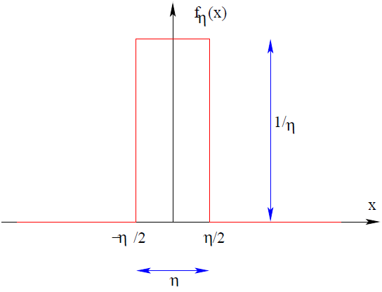
Figure 1: Sketch of $f_{\eta }(x)$. The function is zero everywhere except in a region of width $\eta$ centered at 0, where it equals $1/\eta$. As a result, the integral of this function is 1. If $\eta$ decreases, the function becomes more and more “pointy”.
图 1：$f_{\eta }(x)$ 的示意图。该函数在除“以 0 为中心、宽度为 $\eta$ 的区间”外的所有区域均为 0，在该区间内取值为 $1/\eta$。因此，该函数的积分为 1。当 $\eta$ 减小时，函数图像会变得越来越“尖锐”。

Putting these two facts together, we can basically say that
结合上述两个特性，我们大致可以认为 $\delta (x)$ 满足以下关系：

$$\delta (x)=\{\begin{array}{cc}\infty & ,\text{if }x=0\\ 0& ,\text{otherwise}\end{array}$$

but such that
使得

$${\int }_{-\infty }^{\infty }dx\delta (x)=1$$

This is by no means the only definition of $\delta (x)$. We can also get it as the limit of the continuous functions:
这绝不是 $\delta (x)$ 的唯一定义。我们还可以通过连续函数的极限来定义它：
$$L_{\eta }(x)=\frac{1}{\pi }\frac{\eta }{x^2+{\eta }^2}$$

or

$$G_{\eta }(x)=\frac{1}{\sqrt{2\pi {\eta }^2}}{e}^{-\frac{x^2}{2{\eta }^2}}$$

The first is a so-called Lorentzian, the second is called a Gaussian. Chances are you’ve met them before, in some lab doing error analysis. Both take the highest value when $x=0$ and decrease to zero as $|x|\to \infty$. The constants in front are chosen such that ${\int }_{-\infty }^{\infty }dx{L}_{\eta }(x)={\int }_{-\infty }^{\infty }dx{G}_{\eta }(x)=1$ for any value of $\eta$, so again, the area under each of these curves is precisely 1. Moreover, if you plot them (use Maple to get quick plots) you will see that, again, as $\eta$ decreases, they become pointier too – more narrow but taller. In the limit $\eta \to 0$, they also equal $\delta (x)$. There are many other such examples of ways to define $\delta (x)$.

其中第一个函数称为洛伦兹函数（Lorentzian），第二个函数称为高斯函数（Gaussian）。你很可能在实验室进行误差分析时接触过这两种函数。这两种函数在 $x=0$ 处取得最大值，且当 $|x|\to \infty$ 时均趋近于 0。函数前的常数项经过特殊选取，使得对于任意 $\eta$，都有 ${\int }_{-\infty }^{\infty }dx{L}_{\eta }(x)={\int }_{-\infty }^{\infty }dx{G}_{\eta }(x)=1$，因此这两种函数曲线下的面积也均恰好为 1。此外，若绘制它们的图像（可使用 Maple 软件快速绘图），你会发现：随着 $\eta$ 减小，它们的图像同样会变得更尖锐——宽度更窄、高度更高。当 $\eta \to 0$ 时，这两种函数的极限也等于 $\delta (x)$。除上述方法外，还有许多其他定义 $\delta (x)$ 的方式。

One more interesting definition, which we’ll come back to in a few weeks (when we will understand it as well) is:
还有一种有趣的定义，我们将在几周后（当我们具备足够理解能力时）再深入探讨，其形式如下：

$$\delta (x)=\frac{1}{2\pi }{\int }_{-\infty }^{\infty }{e}^{ikx}dk$$
Why this is so, as I said, will be clear later on. Just for now, you can see that if $x=0$, the integral is indeed infinite, so $\delta (x=0)=\infty$ as required. If $x\ne 0$, you should be able to convince yourselves that the integral equals zero (rewrite $e^{ikx}=\cos (kx)+i\sin (kx)$), then use the fact that $\sin (kx)$ is an odd function so its integral vanishes. And then plot $\cos (kx)$ and consider what area is below this curve if you integrate over all real values). Of course, we’d also need to show that ${\int }_{-\infty }^{\infty }dx\delta (x)=1$ – this will come soon. For the moment, take this as a curiosity.
正如我所说，这种定义的合理性后续会逐步阐明。目前你只需知道：当 $x=0$ 时，该积分的值确实为无穷大，满足 $\delta (x=0)=\infty$ 的要求；当 $x\ne 0$ 时，可通过以下方式证明该积分值为 0——将 $e^{ikx}$ 展开为 $\cos (kx)+i\sin (kx)$，利用“$\sin (kx)$ 是奇函数，其积分值为 0”这一性质，再绘制 $\cos (kx)$ 的图像并分析其在全体实数域上的积分面积。当然，我们还需要证明 ${\int }_{-\infty }^{\infty }dx\delta (x)=1$——这一点后续会补充说明。目前，你只需将这种定义当作一个有趣的知识点了解即可。

Why is this strange function of any use? Well, consider any continuous function $g(x)$ and let’s calculate what is ${\int }_{-\infty }^{\infty }dxg(x)\delta (x-x_0)$. We’ll use the first definition of $\delta (x-x_0)={\lim }_{\eta \to 0}{f}_{\eta }(x-x_0)$. Of course, $f_{\eta }(x-x_0)$ looks just like in Fig.1, except that now it is centered at $x_0$, not at the origin as before. So then:
这种“奇特”的函数为何具有实用性呢？我们不妨以任意连续函数 $g(x)$ 为例，计算积分 ${\int }_{-\infty }^{\infty }dxg(x)\delta (x-x_0)$ 的值。我们将采用第一种定义方式，即 $\delta (x-x_0)={\lim }_{\eta \to 0}{f}_{\eta }(x-x_0)$。显然，$f_{\eta }(x-x_0)$ 的图像与图 1 类似，唯一区别是其峰值中心位于 $x_0$ 处，而非之前的原点。因此可得：
$$\begin{array}{rl}{\int }_{-\infty }^{\infty }dxg(x)f_{\eta }(x-x_0)& ={\int }_{x_0-\frac{\eta }{2}}^{x_0+\frac{\eta }{2}}dxg(x)\frac{1}{\eta }\\ & =\frac{1}{\eta }{\int }_{x_0-\frac{\eta }{2}}^{x_0+\frac{\eta }{2}}dxg(x)\\ & \approx \frac{1}{\eta }\eta g(x_0)=g(x_0)\end{array}$$

where the first equality is because $f_{\eta }(x-x_0)$ vanishes for all values outside $[x_0-\frac{\eta }{2},x_0+\frac{\eta }{2}]$ and equals $\frac{1}{\eta }$ inside this region. The $\approx$ sign becomes exact in the limit $\eta \to 0$. So since this is true for any small $\eta$, it follows that:
上式中第一个等号成立的原因是：$f_{\eta }(x-x_0)$ 在区间 $[x_0-\frac{\eta }{2},x_0+\frac{\eta }{2}]$ 外的所有区域均为 0，在该区间内取值为 $\frac{1}{\eta }$。当 $\eta \to 0$ 时，$\approx$ 可替换为精确的等号。由于上述关系对任意小的 $\eta$ 均成立，因此可得：
$${\int }_{-\infty }^{\infty }dxg(x)\delta \left(x-x_0\right)=g\left(x_0\right)$$

You can think of the delta function like a “spike” that selects the value of $g$ at its location. A graphic depiction of this is shown in the figure below.
你可以将 $\delta$ 函数理解为一个“尖峰”，它能“筛选”出函数 $g$ 在其峰值位置处的取值。下图直观展示了这一特性。

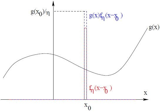
Figure 2: Sketch of some $g(x)$ (black curve), $f_{\eta }(x-x_0)$ (red curve, “spike” centered at $x_0$) and their product (blue dashed curve). The product is also a “spike” centered at $x_0$, of width $\eta$ and of height $g(x_0)/\eta$.
图 2：函数 $g(x)$（黑色曲线）、$f_{\eta }(x-x_0)$（红色曲线，以 $x_0$ 为中心的“尖峰”）及其乘积（蓝色虚线）的示意图。该乘积同样是以 $x_0$ 为中心的“尖峰”，宽度为 $\eta$，高度为 $g(x_0)/\eta$。

Finally, it should be now apparent that if we integrate only over a finite interval, then:
最后，显然若仅在有限区间内积分，则有：

$${\int }_a^{b}dxg(x)\delta \left(x-x_0\right)=\{\begin{array}{cc}g\left(x_0\right)& ,\text{if }a<x_0<b\\ 0& ,\text{otherwise}\end{array}$$

We will use this quite a bit. Note that you can think of ${\int }_{-\infty }^{\infty }dx\delta (x)=1$ as being a particular case of this more general identity, when $g(x)=1$.
这一公式的使用频率很高。需要注意的是，当 $g(x)=1$ 时，${\int }_{-\infty }^{\infty }dx\delta (x)=1$ 可视为上述更一般公式的一个特例。

---

Dirac Delta Functions

狄拉克 $\delta$ 函数

by Dr. Colton, Physics 471 (last updated: 11 Jan 2024)

Definitions

定义

1. Definition as limit. 极限定义

The Dirac delta function can be thought of as a rectangular pulse that grows narrower and narrower while simultaneously growing larger and larger.
狄拉克 $\delta$ 函数可理解为一个“矩形脉冲”：随着脉冲宽度不断变窄，其高度同时不断增大。

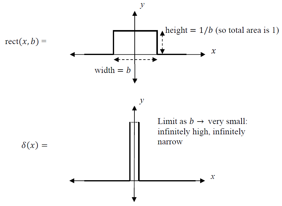
Note that the integral of the delta function is the area under the curve, and has been held constant at 1 throughout the limit process.
需注意，delta 函数的积分即为其曲线下的面积，在整个极限过程中，该面积始终保持为 1。

$${\int }_{-\infty }^{\infty }\delta (x)dx=1$$

Shifting the origin. 原点平移

Just as a parabola can be shifted away from the origin by writing $y=(x-x_0{)}^2$ instead of $y=x^2$, any function can be shifted to the right by writing $x-x_0$ in place of $x$ (here $x_0$ is positive).
正如抛物线可通过将 $y=x^2$ 改写为 $y=(x-x_0{)}^2$ 实现原点平移一样，任意函数均可通过将自变量 $x$ 替换为 $x-x_0$（其中 $x_0$ 为正数）实现向右平移。

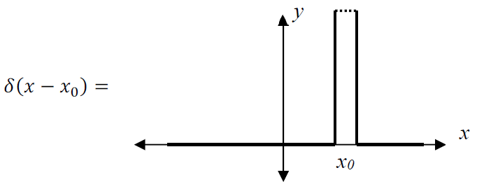
Shifting the position of the peak doesn’t affect the total area if the integral is taken from $-\infty$ to $+\infty$, or if the interval from $a$ to $b$ contains the peak.
若积分区间为 $-\infty$ 到 $+\infty$，或区间 $[a,b]$ 包含 $\delta$ 函数的峰值，则平移峰值位置不会改变积分的总面积。

$${\int }_{-\infty }^{\infty }\delta (x-x_0)dx=1$$

For that matter, since all of the area occurs right in one spot, one can write:
正因如此，由于 $\delta$ 函数的面积集中在单一位置，就有：

$${\int }_a^b\delta (x-x_0)dx=1$$

as long as the interval from $a$ to $b$ contains the delta function peak at $x_0$.
只要区间 $[a,b]$ 包含位于 $x_0$ 处的峰值。

Disclaimer: Mathematicians may object that since the Dirac delta function is only defined in terms of a limit, and/or in terms of how it behaves inside integrals, it is not actually a function but rather a generalized function and/or a functional. While that is technically true, physicists tend to ignore such issues and recognize that for all practical purposes the delta function can be thought of as a very large and very narrow peak at the origin with an integrated area of 1, as I have described it.
免责声明：数学家可能会提出异议：由于狄拉克 $\delta$ 函数仅通过极限或其在积分中的表现来定义，因此它并非真正的函数，而是广义函数（generalized function）或泛函（functional）。尽管从数学严谨性角度而言，这种说法是正确的，但物理学家通常会忽略这类问题，并且认为从实际应用角度出发，delta 函数可按前文描述理解为“位于原点处、高度极大、宽度极窄且积分面积为 1 的尖峰”。

2. Definition as derivative of step function. 阶跃函数导数定义

The step function, also called the “Heaviside step function” is usually defined like this${}^1$:
阶跃函数（又称“ Heaviside 函数”，Heaviside step function）的通常定义为：

$$H(x)=\{\begin{array}{rlr}& 0,& forx<0\\ & 0.5,& forx=0\\ & 1,& forx>0\end{array}$$

1 This is also sometimes called the “theta function” or “Heaviside theta function” and the symbol $\theta (x)$ is often used for the function (𝜃 = capital theta).
1 这有时也被称为 “θ 函数” 或 “Heaviside θ 函数”，符号 $\theta (x)$ 经常用于表示该函数（𝜃 = 大写 theta）。

It’s a function whose only feature is a step up from 0 to 1, at the origin:
该函数的唯一特征是在原点处从 0 跃变到 1：

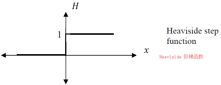
What’s the derivative of this function?

该函数的导数

Well, the slope is zero for $x<0$ and the slope is zero for $x>0$. What about right at the origin? The slope is infinite! So the derivative of this function is a function which is zero everywhere except at the origin, where it’s infinite. Also, the integral of that derivative function from $-\infty$ to $+\infty$ will be $H(\infty )-H(-\infty )$, which is 1! An infinitely narrow, infinitely tall peak at the origin whose integral is 1? That’s the Dirac delta function! Thus $\delta (x)$ can also be defined as the derivative of the Heaviside step function:
对于 $x<0$ 和 $x>0$ 的区域，函数斜率均为 0；而在原点处，斜率为无穷大！因此，该函数的导数满足“除原点外处处为 0，在原点处为无穷大”。此外，该导数在 $-\infty$ 到 $+\infty$ 区间内的积分等于 $H(\infty )-H(-\infty )$，其值为 1！一个“位于原点处、宽度无穷窄、高度无穷大且积分面积为 1 的尖峰”——这正是狄拉克 $\delta$ 函数！因此，$\delta (x)$ 也可定义为 Heaviside 函数的导数：
$$\delta (x)=\frac{dH(x)}{dx}$$

4. Definition as Fourier transform. 傅里叶变换定义

The Fourier transform of a function gives you the frequency components of the function. What do you get when take the Fourier transform of a pure sine or cosine wave oscillating at ${\omega }_0$? There is only one frequency component, so the Fourier transform must be a single, very large peak right at ${\omega }_0$. A delta function !${}^2$
函数的傅里叶变换可给出该函数的频率成分。对以 ${\omega }_0$ 为角频率振荡的纯正弦波或纯余弦波进行傅里叶变换，会得到什么结果呢？由于这类波仅含一个频率成分，其傅里叶变换必然是一个位于 ${\omega }_0$ 处、高度极大的单一尖峰——即 $\delta$ 函数！

2 More technically, F T { cos ⁡ ω 0 t } FT\{\cos \omega_0 t\} FT{cosω0​t} has two real delta function peaks, one at ${\omega }_0$ and one at $-{\omega }_0$, and F T { sin ⁡ ω 0 t } FT\{\sin \omega_0 t\} FT{sinω0​t} has two imaginary peaks, an upward one at $-{\omega }_0$ and a downward one at ${\omega }_0$.
2 更技术性地说， F T { cos ⁡ ω 0 t } FT\{\cos \omega_0 t\} FT{cosω0​t} 有两个实数 $\delta$ 函数峰值，一个在 ${\omega }_0$ 处，一个在 $-{\omega }_0$ 处，而 F T { sin ⁡ ω 0 t } FT\{\sin \omega_0 t\} FT{sinω0​t} 有两个虚数峰值，一个向上的在 $-{\omega }_0$ 处，一个向下的在 ${\omega }_0$ 处。

More technically, F T { cos ⁡ ω 0 t } FT\{\cos\omega_{0}t\} FT{cosω0​t} has two real delta function peaks, one at ${\omega }_0$ and one at $-{\omega }_0$, and F T { sin ⁡ ω 0 t } FT\{\sin\omega_{0}t\} FT{sinω0​t} has two imaginary peaks, an upward one at $-{\omega }_0$ and a downward one at ${\omega }_0$.
更严谨地说， F T { cos ⁡ ω 0 t } FT\{\cos\omega_{0}t\} FT{cosω0​t} 包含两个实 $\delta$ 函数峰值，分别位于 ${\omega }_0$ 和 $-{\omega }_0$ 处；而 F T { sin ⁡ ω 0 t } FT\{\sin\omega_{0}t\} FT{sinω0​t} 包含两个虚数峰值，一个正向峰值位于 $-{\omega }_0$ 处，一个负向峰值位于 ${\omega }_0$ 处。

5. Definition as density. 密度定义

What’s a function which represents the density of a 1 kg point mass located at the origin? Well, it’s a function that must be zero everywhere except at the origin-and it must be infinitely large at the origin because for a mass that truly occupies only a single point, the mass per volume is infinite. How about its integral? The volume integral of the density must give you the mass, which is 1 kg. A function that is zero everywhere except infinite at the origin, and has an integral equal to 1? It’s the Dirac delta function again!
如何用函数表示“位于原点处、质量为 1 千克的点质量”的密度？该函数需满足：除原点外处处为 0，且在原点处为无穷大——因为一个真正仅占据单一质点的质量，其体积密度为无穷大。那么该函数的积分呢？密度的体积分必须等于总质量，即 1 千克。一个“除原点外处处为 0、原点处为无穷大且积分等于 1”的函数——这再次指向了狄拉克 $\delta$ 函数！

More precisely, that last example would be a three-dimensional analog to the regular delta function $\delta (x)$, because the density must be integrated over three dimensions in order to give the mass. This is typically written $\delta (\mathbf{r})$ or as ${\delta }^3(\mathbf{r})$, and is the product of three one-dimensional delta functions:
更精确地说，上述例子对应的是常规一维 $\delta$ 函数 $\delta (x)$ 的三维推广形式，因为密度需要通过三维体积分才能得到总质量。三维 $\delta$ 函数通常记为 $\delta (\mathbf{r})$ 或 ${\delta }^3(\mathbf{r})$，它是三个一维 $\delta$ 函数的乘积：
$${\delta }^3(\mathbf{r})=\delta (x)\delta (y)\delta (z)$$

For a delta function located at ${\mathbf{r}}_0=(x_0,y_0,z_0)$ instead of at the origin, we have:
若 $\delta$ 函数的峰值位于 ${\mathbf{r}}_0=(x_0,y_0,z_0)$（而非原点），则其表达式为：
$${\delta }^3(\mathbf{r}-{\mathbf{r}}_0)=\delta (x-x_0)\delta (y-y_0)\delta (z-z_0)$$

Properties

性质

1. Integral. 积分性质

One of the most important properties of the delta function has already been mentioned: it integrates to
delta 函数最重要的性质之一已在前文提及：其积分值为 1。
$${\int }_{-\infty }^{\infty }\delta (x)dx=1$$

2. Sifting property. 筛选性质

When a delta function $\delta (x-x_0)$ multiplies another function $f(x)$, the product must be zero everywhere except at the location of the infinite peak, $x_0$. At that location the product is infinite like the delta function, but it must be a “larger” or “smaller” infinity, if those terms make sense to use, depending on whether the value of $f(x)$ at that point is larger or smaller than 1. In other words, the area of the product function is not just 1 anymore, it is 1 times the value of $f(x)$ at the infinite peak $x=x_0$. This is called the “sifting property” of the delta function:
当 $\delta$ 函数 $\delta (x-x_0)$ 与另一个函数 $f(x)$ 相乘时，乘积函数除在峰值位置 $x_0$ 处外，其余区域均为 0。在 $x_0$ 处，乘积函数与 $\delta$ 函数一样为无穷大，但这种“无穷大”的“量级”会取决于 $f(x)$ 在 $x_0$ 处的取值（若该表述可理解）：若 $f(x_0)>1$，则乘积函数的“无穷大”量级更大；若 $f(x_0)<1$，则量级更小。换句话说，乘积函数的积分面积不再是 1，而是 1 与 $f(x)$ 在峰值位置 $x=x_0$ 处取值的乘积。这一特性被称为 $\delta$ 函数的“筛选性质”：
$${\int }_{-\infty }^{\infty }\delta \left(x-x_0\right)f(x)dx=f\left(x_0\right)$$

3. Symmetry. 对称性

A few other properties can be readily seen from the definition of the delta function: $\delta (x)$ behaves as if it were an even function.
从 $\delta$ 函数的定义中可直接得出另一个性质：$\delta (x)$ 表现为偶函数。

$$\begin{array}{lcl}\delta (x)=\delta (-x)& & \delta (x)\text{ behaves as if it were an even function}\\ \delta (x-x_0)=\delta (-(x-x_0))& & \delta (x-x_0)\text{ is symmetric about }x=x_0\end{array}$$

4. Linear systems. If a physical system has linear responses and if its response to delta functions (“impulses”) is known, then the output of this system can be determined for almost any input, no matter how complex. This rather amazing property of linear systems is a result of the following: almost any arbitrary function can be decomposed into (or “sampled by”) a linear combination of delta functions, each weighted appropriately, and each of which produces its own impulse response. Thus, by application of the superposition principle, the overall response to an arbitrary input can be found by adding up all of the impulse responses of the sampled values of the function. This is a complicated paragraph, so give it some thought.
   线性系统中的应用。若一个物理系统具有线性响应特性，且其对 $\delta$ 函数（“冲激信号”）的响应已知，则该系统对几乎所有输入（无论多么复杂）的输出均可确定。线性系统的这一出色特性源于以下原理：几乎任意函数都可分解为（或“被采样为”）delta 函数的线性组合（每个 $\delta$ 函数都有适当的权重），且每个 $\delta$ 函数都会产生各自的冲激响应。因此，根据叠加原理，对任意输入的总响应可通过累加函数采样值对应的所有冲激响应得到。这段话的内容较为复杂，请仔细思考理解。

Fourier Transforms

傅里叶变换

1. FT of a single delta function. 单个 $\delta$ 函数的傅里叶变换

The Fourier transform of a single delta function in time can be obtained using the sifting property and the definition of the F.T.:
利用筛选性质和傅里叶变换的定义，可得到时域中单个 $\delta$ 函数的傅里叶变换：
F T { δ ( t ) } = 1 2 π ∫ − ∞ ∞ δ ( t ) e i ω t d t = 1 2 π e i ω ( 0 ) = 1 2 π \begin{aligned} FT\{\delta(t)\} &= \frac{1}{\sqrt{2\pi}} \int_{-\infty}^{\infty} \delta(t) e^{i\omega t} dt \\ &= \frac{1}{\sqrt{2\pi}} e^{i\omega(0)} \\ &= \frac{1}{\sqrt{2\pi}} \end{aligned} FT{δ(t)}​=2π ​1​∫−∞∞​δ(t)eiωtdt=2π ​1​eiω(0)=2π ​1​​
Similarly, the Fourier transform of $\delta (t-t_0)$ is:
同理，$\delta (t-t_0)$ 的傅里叶变换形式如上：

F T { δ ( t − t 0 ) } = 1 2 π ∫ − ∞ ∞ δ ( t − t 0 ) e − i ω t d t = 1 2 π e − i ω t 0 \begin{align*} FT\{\delta (t-{{t}_{0}})\} & =\frac{1}{\sqrt{2\pi }}\int_{-\infty }^{\infty }{\delta }(t-{{t}_{0}}){{e}^{-i\omega t}}dt \\ & =\frac{1}{\sqrt{2\pi }}{{e}^{-i\omega {{t}_{0}}}} \end{align*} FT{δ(t−t0​)}​=2π ​1​∫−∞∞​δ(t−t0​)e−iωtdt=2π ​1​e−iωt0​​

The Fourier transform of $\delta (t-t_0)$, which by definition is a function of $\omega$, has a constant amplitude but phase that varies linearly with $\omega$.
根据定义，$\delta (t-t_0)$ 的傅里叶变换是关于 $\omega$ 的函数，其振幅恒定，相位随 $\omega$ 线性变化。

Another interesting way to define the delta function can be obtained by doing the reverse Fourier transform and setting it equal to the original delta function:
通过逆傅里叶变换并令其等于原 $\delta$ 函数，可得到 $\delta$ 函数的另一种有趣定义：
$$\begin{array}{rl}\delta (t-t_0)& =F{T}^{-1}\left\{\frac{1}{\sqrt{2\pi }}{e}^{i\omega t_0}\right\}\\ & =\frac{1}{\sqrt{2\pi }}{\int }_{-\infty }^{\infty }\left(\frac{1}{\sqrt{2\pi }}{e}^{i\omega t_0}\right)e^{-i\omega t}d\omega \\ & =\frac{1}{2\pi }{\int }_{-\infty }^{\infty }{e}^{-i\omega (t-t_0)}d\omega \end{array}$$

yet another way the Dirac delta function can be defined
狄拉克函数的另一种定义方式

Note: the negative sign in the exponent is optional for this definition, as can be seen by substituting ${\omega }^{\prime }=-\omega$; the limits get reversed but a negative sign gets added since $d{\omega }^{\prime }=-d\omega$, so the integral $\frac{1}{2\pi }{\int }_{-\infty }^{\infty }{e}^{i\omega (t-t_0)}d\omega$ is equal to the integral with the negative exponent.
注：该定义中指数的负号可任选。令 ${\omega }^{\prime }=-\omega$ 即可验证：积分上下限会反转，但由于 $d{\omega }^{\prime }=-d\omega$，会引入一个负号，因此积分 $\frac{1}{2\pi }{\int }_{-\infty }^{\infty }{e}^{i\omega (t-t_0)}d\omega$ 与指数带负号的积分值相等。

3. FT of two delta functions. 两个 $\delta$ 函数的傅里叶变换

As another short example, let’s calculate the (spatial) Fourier transform of two delta functions centered on the origin, separated by a distance $d$. One is at $x=-d/2$ and the other is at $x=+d/2$, therefore:
作为另一个简单例子，我们来计算两个“以原点为中心、间距为 $d$”的 $\delta$ 函数的（空间）傅里叶变换。其中一个 $\delta$ 函数位于 $x=-d/2$ 处，另一个位于 $x=+d/2$ 处，因此（两个 $\delta$ 函数）其傅里叶变换为：
F T { t w o   d e l t a s } = 1 2 π ∫ − ∞ ∞ ( δ ( x + d 2 ) + δ ( x − d 2 ) ) e i k x d x = 1 2 π ( e i k ( − d 2 ) + e i k ( d 2 ) ) = 1 2 π ( 2 cos ⁡ ( k d 2 ) ) = 2 / π cos ⁡ ( k d 2 ) \begin{aligned} FT\{two\ deltas\} & =\frac{1}{\sqrt{2 \pi}} \int_{-\infty}^{\infty}\left(\delta\left(x+\frac{d}{2}\right)+\delta\left(x-\frac{d}{2}\right)\right) e^{i k x} d x \\ & =\frac{1}{\sqrt{2 \pi}}\left(e^{i k\left(-\frac{d}{2}\right)}+e^{i k\left(\frac{d}{2}\right)}\right) \\ & =\frac{1}{\sqrt{2 \pi}}\left(2 \cos \left(\frac{k d}{2}\right)\right) \\ & =\sqrt{2 / \pi} \cos \left(\frac{k d}{2}\right) \end{aligned} FT{two deltas}​=2π ​1​∫−∞∞​(δ(x+2d​)+δ(x−2d​))eikxdx=2π ​1​(eik(−2d​)+eik(2d​))=2π ​1​(2cos(2kd​))=2/π ​cos(2kd​)​

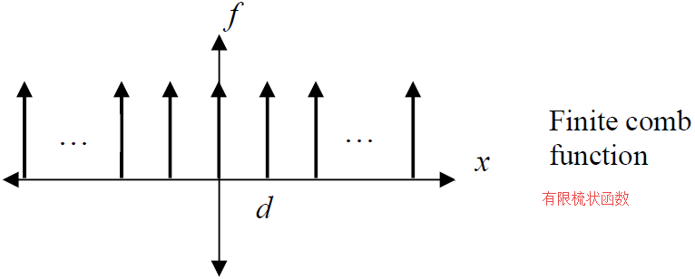
4. FT of a finite Dirac comb. 有限狄拉克梳状函数的傅里叶变换

An infinite number of equally spaced delta functions is called a Dirac comb. A finite comb function with a delta function at the origin, $N$ delta functions to the left of the origin, and $N$ delta functions to the right of the origin, has $2N+1$ total delta functions and can be written as:
无穷多个等间距排列的 $\delta$ 函数称为狄拉克梳状函数（Dirac comb）。一个“在原点处有一个 $\delta$ 函数、原点左侧有 $N$ 个 $\delta$ 函数、原点右侧有 $N$ 个 $\delta$ 函数”的有限梳状函数，总共有 $2N+1$ 个 $\delta$ 函数，其表达式可写为：
$$com{b}_N(x)=\sum _{j=-N}^N\delta (x-x_j)$$

where $x_j=jd$, with $d$ being the spacing between delta functions.
其中 $x_j=jd$，$d$ 为 $\delta$ 函数之间的间距。

As is mentioned in the Wikipedia article, https://en.wikipedia.org/wiki/Dirac_comb, one potential use for the comb function is as a sampling function (see “Linear systems,” above).
如维基百科文章所述，梳状函数的一个潜在用途是作为采样函数。

The Fourier transform of the comb function is:
该梳状函数的傅里叶变换为：
FT { comb N ( x ) } = 1 2 π ∫ − ∞ ∞ ∑ j = − N N δ ( x − x j ) e i k x d x = 1 2 π ∑ j = − N N e i k x j \begin{align*} \text{FT}\{\text{comb}_N(x)\} &= \frac{1}{\sqrt{2\pi}} \int_{-\infty}^{\infty} \sum_{j=-N}^{N} \delta(x - x_j) e^{ikx} dx \\ &= \frac{1}{\sqrt{2\pi}} \sum_{j=-N}^{N} e^{ikx_j} \end{align*} FT{combN​(x)}​=2π ​1​∫−∞∞​j=−N∑N​δ(x−xj​)eikxdx=2π ​1​j=−N∑N​eikxj​​

which, after summing the finite series, doing some algebra, and putting things in terms of the comb spacing $d$ and the total number of delta functions $N_{tot}=2N+1$, reduces to:
对有限级数求和、进行代数运算，并结合梳状函数间距 $d$ 和 $\delta$ 函数总数 $N_{tot}=2N+1$，可将上式化简为：

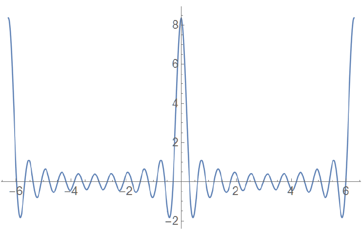
F T { c o m b N ( x ) } = 1 2 π sin ⁡ ( N t o t k d 2 ) sin ⁡ ( k d 2 ) F T\left\{comb_{N}(x)\right\}=\frac{1}{\sqrt{2 \pi}} \frac{\sin \left(\frac{N_{tot } k d}{2}\right)}{\sin \left(\frac{k d}{2}\right)} FT{combN​(x)}=2π ​1​sin(2kd​)sin(2Ntot​kd​)​

That is a periodic function made up of large primary peaks surrounded by secondary peaks that decrease in amplitude as you move away from the primary peak.
这是一个由大型主峰组成的周期函数，主峰周围有次级峰，当你远离主峰时，次级峰的振幅会逐渐减小。

F T { c o m b N ( x ) } FT\{comb_{N}(x)\} FT{combN​(x)} plotted here as a function of $k$, for $N_{tot}=21$ and $d=1$.
这里的 F T { c o m b N ( x ) } FT\{comb_{N}(x)\} FT{combN​(x)} 作为 $k$ 的函数绘制出来，其中 $N_{tot}=21$，$d=1$。

Notice that the function of $k$ is periodic and repeats every $2\pi /d$.
需注意，该关于 $k$ 的函数具有周期性，周期为 $2\pi /d$。

As can be found from L’Hospital’s Rule, the amplitude of the primary peak depends on $N_{tot}$:
根据洛必达法则，主峰的幅度取决于 $N_{\text{tot}}$：
$$\text{amplitude}=\frac{1}{\sqrt{2\pi }}{N}_{\text{tot}}$$

The position of the first zero (a measure of the width of the primary peak) is given by:
第一个零点的位置（主峰宽度的度量）由以下公式给出：
$$k_{\text{first zero}}=\frac{2\pi }{N_{\text{tot}}d}$$

5. FT of an infinite Dirac comb function: 无限狄拉克梳状函数的傅里叶变换

Using the previous two equations, one can see that in the limit as $N_{tot}\to \infty$, the large peaks (like the ones at $-2\pi$, 0, and $2\pi$) get infinitely tall and infinitely narrow. They are delta functions! Thus, the Fourier transform of an infinite comb function in $x$ is an infinite comb function in $k$.
结合前两个公式可知，当 $N_{tot}\to \infty$ 时，那些较大的峰值（如位于 $-2\pi$、0 和 $2\pi$ 处的峰值）会变得高度无穷大、宽度无穷窄——它们成为了 $\delta$ 函数！因此，时域 $x$ 中的无限梳状函数，其傅里叶变换是频域 $k$ 中的无限梳状函数。

Explanations and Derivation Details

解释和推导

I. Verification of the Limit Definition of the Delta Function

一、Delta 函数极限定义的验证
As mentioned earlier, $\delta (x)$ can be defined through the limits of rectangular pulses, Lorentzians, and Gaussians. Here, the specific form and verification process of the Lorentzian function are supplemented:
前文提及可通过矩形脉冲、洛伦兹函数（Lorentzian）和高斯函数（Gaussian）的极限定义 $\delta (x)$，此处补充洛伦兹函数的具体形式与验证过程：

The expression for the Lorentzian function is $L_{\eta }(x)=\frac{\eta }{\pi (x^2+{\eta }^2)}$. Integrate it over the entire real number domain:
洛伦兹函数的表达式为 $L_{\eta }(x)=\frac{\eta }{\pi (x^2+{\eta }^2)}$。对其在全体实数域积分：
$${\int }_{-\infty }^{\infty }{L}_{\eta }(x)dx=\frac{\eta }{\pi }{\int }_{-\infty }^{\infty }\frac{1}{x^2+{\eta }^2}dx$$

Let $x=\eta \tan \theta$ (substitution method), then $dx=\eta {\sec }^2\theta d\theta$, and the limits of integration change from $\theta =-\pi /2$ to $\theta =\pi /2$. Substituting these into the integral:
令 $x=\eta \tan \theta$（换元法），则 $dx=\eta {\sec }^2\theta d\theta$，积分上下限变为 $\theta =-\pi /2$ 到 $\theta =\pi /2$，代入后：
$$\frac{\eta }{\pi }{\int }_{-\pi /2}^{\pi /2}\frac{\eta {\sec }^2\theta }{{\eta }^2{\tan }^2\theta +{\eta }^2}d\theta =\frac{1}{\pi }{\int }_{-\pi /2}^{\pi /2}d\theta =1$$

It can be seen that the integral of the Lorentzian function is always 1, satisfying the area condition of the delta function. When $\eta \to 0$, the peak value of $L_{\eta }(x)$ at $x=0$ (which is $\frac{1}{\pi \eta }$) tends to infinity, and at $x\ne 0$, it tends to 0, which conforms to the definition of $\delta (x)$.
可见洛伦兹函数的积分始终为 1，满足 $\delta$ 函数的面积条件。当 $\eta \to 0$ 时，$L_{\eta }(x)$ 在 $x=0$ 处的峰值 $\frac{1}{\pi \eta }$ 趋于无穷大，在 $x\ne 0$ 处趋于 0，符合 $\delta (x)$ 的定义。

II. Extended Physical Significance of the 3D Delta Function

二、三维 $\delta$ 函数的物理意义延伸

The 3D delta function ${\delta }^3(\mathbf{r}-{\mathbf{r}}_0)=\delta (x-x_0)\delta (y-y_0)\delta (z-z_0)$, whose core purpose is to describe the density distribution of “point sources”. For example:
三维 $\delta$ 函数 ${\delta }^3(\mathbf{r}-{\mathbf{r}}_0)=\delta (x-x_0)\delta (y-y_0)\delta (z-z_0)$，其核心用途是描述“点源”的密度分布，例如：

• Charge Density of a Point Charge: If there is a point charge with charge quantity $Q$ at position ${\mathbf{r}}_0$, its charge density $\rho (\mathbf{r})$ can be expressed as $\rho (\mathbf{r})=Q{\delta }^3(\mathbf{r}-{\mathbf{r}}_0)$. Integrating this density over the entire space gives the total charge quantity:
  点电荷的电荷密度：若在位置 ${\mathbf{r}}_0$ 处存在电荷量为 $Q$ 的点电荷，其电荷密度 $\rho (\mathbf{r})$ 可表示为 $\rho (\mathbf{r})=Q{\delta }^3(\mathbf{r}-{\mathbf{r}}_0)$。对该密度在全空间积分，可得到总电荷量：
  $${\int }_{\text{Entire Space 全空间}}\rho (\mathbf{r})dV=Q{\int }_{\text{Entire Space}}{\delta }^3(\mathbf{r}-{\mathbf{r}}_0)dV=Q$$

• Mass Density of a Point Mass: Similarly, for a point mass with mass $m$ at position ${\mathbf{r}}_0$, its mass density ${\rho }_m(\mathbf{r})=m{\delta }^3(\mathbf{r}-{\mathbf{r}}_0)$, and the result of integrating over the entire space is the total mass $m$.
  点质量的质量密度：类似地，位置 ${\mathbf{r}}_0$ 处质量为 $m$ 的点质量，其质量密度 ${\rho }_m(\mathbf{r})=m{\delta }^3(\mathbf{r}-{\mathbf{r}}_0)$，全空间积分结果为总质量 $m$。

III. Specific Application of the Sampling Property of the Dirac Comb Function

三、狄拉克梳状函数采样性质的具体应用

The document points out that the Dirac comb function can be used as a “sampling function”, which essentially utilizes the periodicity of the comb function and the sifting property of the delta function to achieve discrete sampling of continuous functions. Let the continuous function be $f(x)$ and the sampling interval be $d$; then the sampling process can be expressed as:
文档指出狄拉克梳状函数可作为“采样函数”，其本质是利用梳状函数的周期性与 $\delta$ 函数的筛选性，实现对连续函数的离散采样。设连续函数为 $f(x)$，采样间隔为 $d$，则采样过程可表示为：
$$f_{\text{Sampled 采样}}(x)=f(x)\cdot com{b}_{\infty }(x)=f(x)\sum _{n=-\infty }^{\infty }\delta (x-nd)$$

According to the sifting property of the delta function, $f(x)\delta (x-nd)=f(nd)\delta (x-nd)$; therefore:
根据 $\delta$ 函数的筛选性质，$f(x)\delta (x-nd)=f(nd)\delta (x-nd)$，因此：
$$f_{\text{Sampled 采样}}(x)=\sum _{n=-\infty }^{\infty }f(nd)\delta (x-nd)$$

This formula shows that the sampling result is a series of delta functions located at $x=nd$ (where $n$ is an integer) with intensities equal to $f(nd)$, which exactly correspond to the values of the continuous function at discrete points. This property is the mathematical basis of the “sampling theorem” in digital signal processing.
该式表明，采样结果是一系列位于 $x=nd$（$n$ 为整数）处、强度为 $f(nd)$ 的 $\delta$ 函数，恰好对应连续函数在离散点上的取值。这一性质是数字信号处理中“采样定理”的数学基础。

IV. Comparison of Fourier Transforms Between Finite and Infinite Dirac Comb Functions

四、有限与无限狄拉克梳状函数傅里叶变换的差异对比

Characteristic 特性	Finite Dirac Comb Function ($N_{\text{tot}}=2N+1$) 有限狄拉克梳状函数（$N_{\text{tot}}=2N+1$）	Infinite Dirac Comb Function ($N_{\text{tot}}\to \infty$) 无限狄拉克梳状函数（$N_{\text{tot}}\to \infty$）
Form of Fourier Transform 傅里叶变换形式	$\frac{1}{\sqrt{2\pi }}\frac{\sin \left(\frac{N_{\text{tot}}kd}{2}\right)}{\sin \left(\frac{kd}{2}\right)}$	$\frac{2\pi }{d}{\sum }_{n=-\infty }^{\infty }\delta \left(k-\frac{2\pi n}{d}\right)$
Shape in Frequency Domain 频率域形态	Main peak + side lobes (amplitude of side lobes decays with $k$) 主峰值+旁瓣（旁瓣振幅随 $k$ 衰减）	Equally spaced delta functions (no side lobes, only discrete peaks) 等间距的 $\delta$ 函数（无旁瓣，仅离散峰值）
Periodicity 周期性	Non-strict periodicity (interval between main peaks is $2\pi /d$, but side lobes disrupt periodicity) 非严格周期（主峰值间隔为 $2\pi /d$，但旁瓣破坏周期性）	Strict periodicity (period is $2\pi /d$) 严格周期（周期为 $2\pi /d$）
Application Scenario 应用场景	Sampling and spectrum analysis of finite-length signals 有限长度信号的采样与频谱分析	Spectrum representation of infinite periodic signals (e.g., digital clock signals) 无限长周期信号的频谱表示（如数字时钟信号）

For example, when $N_{\text{tot}}=5$ (i.e., 5 delta functions) and $d=1$, the Fourier transform of the finite comb function has a main peak at $k=0$, zeros at $k=\pm 2\pi /5,\pm 4\pi /5$, and side lobes between the zeros. In contrast, the Fourier transform of the infinite comb function only has sharp delta peaks at $k=\pm 2\pi n$ (where $n$ is an integer), with no side lobe interference.
例如，当 $N_{\text{tot}}=5$（即 5 个 $\delta$ 函数）、$d=1$ 时，有限梳状函数的傅里叶变换在 $k=0$ 处有主峰值，在 $k=\pm 2\pi /5,\pm 4\pi /5$ 处有零点，零点之间存在旁瓣；而无限梳状函数的傅里叶变换仅在 $k=\pm 2\pi n$（$n$ 为整数）处有尖锐的 delta 峰值，无旁瓣干扰。

---

狄拉克梳状函数的傅里叶变换

phoenix@Capricornus 发布时间：2025-04-22 12:57:06

1. 时域冲激串序列

时域冲激串序列的表达式为：
$$p(t)=\sum _{n=-\infty }^{\infty }\delta (t-nT)$$
其中，$p(t)$ 称为冲激串序列，其具有周期性，周期为 $T$。

2. 冲激串序列的傅里叶级数展开

由于 $p(t)$ 是周期信号，可将其展开为傅里叶级数，形式如下：
$$p(t)=\sum _{n=-\infty }^{\infty }\delta (t-nT)=\sum _{k=-\infty }^{\infty }P(k{\Omega }_0)e^{jk{\Omega }_{0}t}$$

2.1 傅里叶系数计算

傅里叶系数 $P(k{\Omega }_0)$ 的求解需利用狄拉克 delta 函数的筛选性质，计算过程如下：
$$P(k{\Omega }_0)=\frac{1}{T}{\int }_{-T/2}^{T/2}\delta (t)e^{-jk{\Omega }_{0}t}dt=\frac{1}{T}$$
（注：因 $\delta (t)$ 仅在 $t=0$ 处有值，积分区间 $[-T/2,T/2]$ 包含 $t=0$，故积分结果为 $\delta (0)$ 与 $e^0$ 的乘积，最终简化为 $\frac{1}{T}$）

2.2 傅里叶级数展开结果

将傅里叶系数代入级数表达式，可得：
$$\sum _{n=-\infty }^{\infty }\delta (t-nT)=\frac{1}{T}\sum _{k=-\infty }^{\infty }{e}^{jk{\Omega }_{0}t}$$
其中，${\Omega }_0=\frac{2\pi }{T}$（${\Omega }_0$ 为基波角频率，与周期 $T$ 成反比）。

3. 冲激串序列的傅里叶变换

对 $p(t)$ 的傅里叶级数展开式求傅里叶变换，步骤如下：

3.1 变换过程

$$P(j\Omega )={\int }_{-\infty }^{\infty }\underset{p(t)}{\underbrace{\frac{1}{T}\sum _{k=-\infty }^{\infty }{e}^{jk{\Omega }_{0}t}}}{e}^{-j\Omega t}dt$$
利用积分与求和的交换律，可拆分表达式：
$$P(j\Omega )=\frac{1}{T}\sum _{k=-\infty }^{\infty }{\int }_{-\infty }^{\infty }{e}^{jk{\Omega }_{0}t}{e}^{-j\Omega t}dt$$

3.2 关键性质：复指数信号的傅里叶变换

对于单个复指数信号 $x(t)=e^{j{\Omega }_{0}t}$，其傅里叶变换为：
$$x(t)=e^{j{\Omega }_{0}t}\iff X(j\Omega )=2\pi \delta (\Omega -{\Omega }_0)$$

• 时域含义：$x(t)=e^{j{\Omega }_{0}t}$ 是角频率为 ${\Omega }_0$ 的复指数信号；
• 频域含义：$X(j\Omega )=2\pi \delta (\Omega -{\Omega }_0)$ 表示频域中仅在 $\Omega ={\Omega }_0$ 处存在冲激（谱线），幅度为 $2\pi$。

3.3 最终变换结果

将复指数信号的傅里叶变换代入 $P(j\Omega )$ 的表达式，可得：
$$P(j\Omega )=\frac{2\pi }{T}\sum _{k=-\infty }^{\infty }\delta (\Omega -k{\Omega }_0)$$

即时域冲激串与频域冲激串的傅里叶变换对为：
$$\sum _{n=-\infty }^{\infty }\delta (t-nT)\iff \frac{2\pi }{T}\sum _{k=-\infty }^{\infty }\delta (\Omega -k{\Omega }_0)$$

4. 结论

1. 时域与频域的对应关系：时域的周期冲激串（周期为 $T$），其傅里叶变换是频域的周期冲激串（间隔为 ${\Omega }_0$）；
2. 参数的反比关系：时域冲激的间距 $T$ 与频域冲激的间距 ${\Omega }_0$ 满足 ${\Omega }_0=\frac{2\pi }{T}$，二者成反比；
3. 重要应用：该变换对是信号处理中“采样定理”的核心数学基础，广泛用于模数转换（ADC）、信号重构等场景。

---

狄拉克 $\delta$ 函数(Dirac delta)和狄拉克梳状函数(Dirac comb)

wymanth Written on October 18, 2015

狄拉克 $\delta$ 函数(Dirac delta)的定义

$$\delta (t)=\{\begin{array}{ll}+\infty ,& t=0\\ 0,& t\ne 0\end{array}$$
且满足积分条件：
$${\int }_{-\infty }^{\infty }\delta (t)dt=1$$

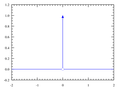
δ 函数波形图，横轴范围为 -2 至 2，纵轴范围为 -0.2 至 1.2，图中显示 t=0 时函数值趋近于 +∞，t≠0 时函数值为 0。

狄拉克 $\delta$ 函数的性质

1. 对称性质

从 $\delta$ 函数的波形图（或定义）可直观看出， $\delta$ 函数为偶函数，即：
$$\delta (t)=\delta (-t)$$

2. 缩放性质

设常数为 $a$，令 $u=at$，结合 $\delta$ 函数的积分特性可得：
$$dt=\frac{1}{a}du$$
$${\int }_{-\infty }^{\infty }\delta (at)dt={\int }_{-\infty }^{\infty }\delta (u)\cdot \frac{1}{a}du=\frac{1}{a}{\int }_{-\infty }^{\infty }\delta (u)du=\frac{1}{a}$$
由此推出：
$$\delta (at)=\frac{1}{a}\delta (t)$$
又因 $\delta$ 函数的对称性质，最终可得：
$$\delta (at)=\frac{1}{|a|}\delta (t)$$

3. 代数性质

$$t\delta (t)=0$$
该性质可从 $\delta$ 函数的基本定义直接推导，证明过程较为简单。

4. 平移性质

$${\int }_{-\infty }^{\infty }f(t)\delta (t-T)dt=f(T)$$
可通过 $\delta$ 函数的定义直观理解此性质。

5. $\delta$ 函数的傅里叶变换

$$\mathcal{F}[\delta (s)]={\int }_{-\infty }^{\infty }{e}^{-2\pi ist}\delta (t)=1$$
由于仅当 $t=0$ 时， $\delta$ 函数非 0（此时取值可理解为满足积分条件的特殊值），因此上述积分结果为 1。 $\delta$ 函数的傅里叶变换是常数 1，这一性质具有特殊性。

狄拉克梳状函数(Dirac comb)

狄拉克梳状函数在电子工程（electrical engineering）领域，常被称为脉冲序列（impulse train）或采样函数（sampling function）；部分文献中也将其称为 Shah 函数。

其本质是由狄拉克 $\delta$ 函数以周期 $T$ 为间隔构成的无穷级数（即多个 $\delta$ 函数的叠加）。维基百科原文描述为：“A Dirac comb is an infinite series of Dirac delta functions spaced at intervals of T”。
狄拉克梳是以 $T$ 为间隔的狄拉克函数的无穷级数。

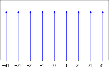
狄拉克梳状函数示意图，每个横轴标注点处均有一个垂直向上的脉冲，代表 δ 函数

狄拉克梳状函数的公式表示

$${\text{III}}_T(t)=\sum _{k=-\infty }^{\infty }\delta (t-kT)$$
该公式与上述示意图完全对应，其中 $k$ 为整数，$T$ 为 $\delta$ 函数的间隔周期。

狄拉克梳状函数的性质

1. 缩放性质

当周期 $T=1$（单位周期）时，狄拉克梳状函数可表示为：
$$\text{III}(t)=\sum _{k=-\infty }^{\infty }\delta (t-k)$$
若对变量 $t$ 缩放 $a$ 倍（即替换为 $at$），则：
$$\text{III}(at)=\sum _{k=-\infty }^{\infty }\delta (at-k)$$
结合 $\delta$ 函数的对称性质公式 $\delta (at)=\frac{1}{a}\delta (t)$，进一步推导：
$$\text{III}(at)=\sum _{k=-\infty }^{\infty }\delta \left(a\left(t-\frac{k}{a}\right)\right)=\sum _{k=-\infty }^{\infty }\frac{1}{a}\delta \left(t-\frac{k}{a}\right)=\frac{1}{a}{\text{III}}_{\frac{1}{a}}(t)$$
即：
$$\text{III}(at)=\frac{1}{a}{\text{III}}_{\frac{1}{a}}(t)$$
也可表示为：
$${\text{III}}_a(t)=\frac{1}{a}\text{III}\left(\frac{t}{a}\right)$$

2. 傅里叶变换

标准狄拉克梳状函数 ${\text{III}}_T(t)$ 的傅里叶变换公式修正为：
$$\mathcal{F}[{\text{III}}_T(t)]=\frac{1}{T}\sum _{k=-\infty }^{\infty }\delta \left(s-\frac{k}{T}\right)$$
该结果表明，狄拉克梳状函数的傅里叶变换仍为狄拉克梳状函数，其周期为 $\frac{1}{T}$（与原函数周期 $T$ 成反比），幅度为 $\frac{1}{T}$。

---

via:

• The Dirac delta function – a quick introduction
  https://phas.ubc.ca/~berciu/TEACHING/PHYS312/LECTURES/FILES/dirac.pdf
• Dirac delta functions
  https://physics.byu.edu/faculty/colton/docs/phy471-resources/Dirac-delta-functions.pdf
• 狄拉克梳状函数的傅里叶变换-优快云博客
  https://blog.youkuaiyun.com/u013600306/article/details/147413924
• 狄拉克 $\delta$ 函数(Dirac delta)和狄拉克梳状函数(Dirac comb)
  https://wyman1024.github.io/shah-function/
• 广义函数_百度百科
  https://baike.baidu.com/item/广义函数/7689493