【MTSP问题算法】基于开普勒优化算法KOA求解单仓库多旅行商问题

 ✅作者简介：热爱科研的Matlab仿真开发者，修心和技术同步精进，

代码获取、论文复现及科研仿真合作可私信。

🍎个人主页：Matlab科研工作室

🍊个人信条：格物致知。

更多Matlab完整代码及仿真定制内容点击👇

智能优化算法       神经网络预测       雷达通信      无线传感器        电力系统

信号处理              图像处理               路径规划       元胞自动机        无人机

🔥 内容介绍

1. 问题描述

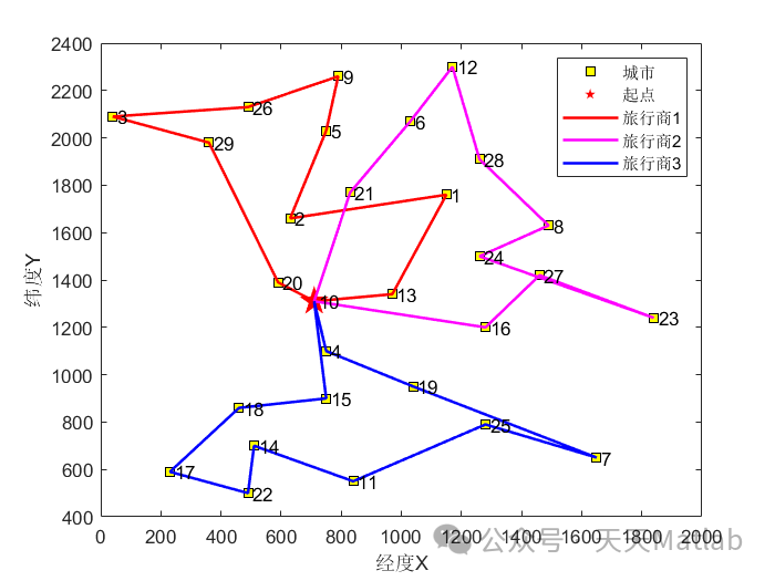
单仓库多旅行商问题（STSP）是经典的组合优化问题之一，它在物流配送、车辆调度等领域有着广泛的应用。STSP的目标是寻找一条最优路径，使得从一个仓库出发，依次访问多个客户点，并最后返回仓库，同时满足以下约束条件：

• 每条路径必须从仓库出发并返回仓库。

• 每条路径必须访问所有客户点一次且仅一次。

• 每条路径的总距离或总成本必须最小。

2. 开普勒优化算法（KOA）

开普勒优化算法（KOA）是一种基于开普勒定律的元启发式算法，它于2016年由李建平等人提出。KOA算法模拟了行星绕太阳运行的运动，将每个待优化问题的解表示为一个行星，并将目标函数值表示为行星与太阳之间的距离。在迭代过程中，KOA算法通过调整行星的位置来不断优化目标函数值，最终找到最优解。

3. 基于KOA算法求解STSP

为了利用KOA算法求解STSP，需要将STSP问题转化为一个优化问题。具体步骤如下：

1. 将仓库和客户点表示为二维空间中的点。

2. 将STSP问题转化为一个最小化总距离的优化问题。

3. 将KOA算法应用于优化问题，并不断调整行星的位置来优化目标函数值。

4. 当KOA算法收敛时，将最优行星的位置转换为最优路径。

📣 部分代码

%_________________________________________________________________________%%  Kepler optimization algorithm (KOA) source codes demo 1.0               %%   Main paper: Abdel-Basset, M., Mohamed, R.                                    %%               Kepler optimization algorithm: A new metaheuristic algorithm inspired by Kepler抯 laws of planetary motion                         %%               Knowledge-Based Systems%               DOI: doi.org/10.1016/j.knosys.2023.110454                 %%_________________________________________________________________________%​​% The Kepler Optimization Algorithmfunction [Sun_Score,Sun_Pos,Convergence_curve]=KOA(SearchAgents_no,Tmax,lb,ub,dim,fobj)​%%%%-------------------Definitions--------------------------%%%%ub=ub.*ones(1,dim);lb=lb.*ones(1,dim);Sun_Pos=zeros(1,dim); % A vector to include the best-so-far Solution, representing the SunSun_Score=inf; % A Scalar variable to include the best-so-far scoreConvergence_curve=zeros(1,Tmax);​%%-------------------Controlling parameters--------------------------%%%%Tc=3;M0=0.1;lambda=15;%% Step 1: Initialization process%%---------------Initialization----------------------%% % Orbital Eccentricity (e)   orbital=rand(1,SearchAgents_no); %% Eq.(4) %% Orbital Period (T) T=abs(randn(1,SearchAgents_no)); %% Eq.(5)Positions=initialization(SearchAgents_no,dim,ub,lb); % Initialize the positions of planetst=0; %% Function evaluation counter %%%%---------------------Evaluation-----------------------%%for i=1:SearchAgents_no    PL_Fit(i)=fobj(Positions(i,:));    % Update the best-so-far solution    if PL_Fit(i)<Sun_Score % Change this to > for maximization problem       Sun_Score=PL_Fit(i); % Update the best-so-far score       Sun_Pos=Positions(i,:); % Update te best-so-far solution    endend​while t<Tmax %% Termination condition   [Order] = sort(PL_Fit);  % Sorting the fitness values of the solutions in current population %% The worst Fitness value at function evaluation t worstFitness = Order(SearchAgents_no); %% Eq.(11) M=M0*(exp(-lambda*(t/Tmax))); %% Eq. (12) %% Computer R that represents the Euclidian distance between the best-so-far solution and the ith solution for i=1:SearchAgents_no    R(i)=0;    for j=1:dim       R(i)=R(i)+(Sun_Pos(j)-Positions(i,j))^2; %% Eq.(7)    end    R(i)=sqrt(R(i)); end %% The mass of the Sun and object i at time t is computed as follows: for i=1:SearchAgents_no    sum=0;    for k=1:SearchAgents_no        sum=sum+(PL_Fit(k)-worstFitness);    end    MS(i)=rand*(Sun_Score-worstFitness)/(sum); %% Eq.(8)    m(i)=(PL_Fit(i)-worstFitness)/(sum); %% Eq.(9) end  %% Step 2: Defining the gravitational force (F) % Computing the attraction force of the Sun and the ith planet according to the universal law of gravitation: for i=1:SearchAgents_no    Rnorm(i)=(R(i)-min(R))/(max(R)-min(R)); %% The normalized R (Eq.(24))    MSnorm(i)=(MS(i)-min(MS))/(max(MS)-min(MS)); %% The normalized MS    Mnorm(i)=(m(i)-min(m))/(max(m)-min(m)); %% The normalized m    Fg(i)=orbital(i)*M*((MSnorm(i)*Mnorm(i))/(Rnorm(i)*Rnorm(i)+eps))+(rand); %% Eq.(6) end %% a1 represents the semimajor axis of the elliptical orbit of object i at time t, for i=1:SearchAgents_no    a1(i)=rand*(T(i)^2*(M*(MS(i)+m(i))/(4*pi*pi)))^(1/3); %% Eq.(23) end  for i=1:SearchAgents_no    %% a2 is a cyclic controlling parameter that is decreasing gradually from -1 to ?2    a2=-1+-1*(rem(t,Tmax/Tc)/(Tmax/Tc)); %% Eq.(29)    %% ? is a linearly decreasing factor from 1 to ?2    n=(a2-1)*rand+1; %% Eq.(28)    a=randi(SearchAgents_no);  %% An index of a solution selected at random    b=randi(SearchAgents_no); %% An index of a solution selected at random    rd=rand(1,dim); %% A vector generated according to the normal distribution    r=rand; %% r1 is a random number in [0,1]    %% A randomly-assigned binary vector     U1=rd<r; %% Eq.(21)      O_P=Positions(i,:); %% Storing the current position of the ith solution    %% Step 6: Updating distance with the Sun    if rand<rand         %% h is an adaptive factor for controlling the distance between the Sun and the current planet at time t         h=(1/(exp(n.*randn))); %% Eq.(27)         %% An verage vector based on three solutions: the Current solution, best-so-far solution, and randomly-selected solution         Xm=(Positions(b,:)+Sun_Pos+Positions(i,:))/3.0;          Positions(i,:)=Positions(i,:).*U1+(Xm+h.*(Xm-Positions(a,:))).*(1-U1); %% Eq.(26)    else                %% Step 3: Calculating an object?velocity        % A flag to opposite or leave the search direction of the current planet         if rand<0.5 %% Eq.(18)           f=1;         else           f=-1;         end         L=(M*(MS(i)+m(i))*abs((2/(R(i)+eps))-(1/(a1(i)+eps))))^(0.5); %% Eq.(15)         U=rd>rand(1,dim); %% A binary vector         if Rnorm(i)<0.5 %% Eq.(13)            M=(rand.*(1-r)+r); %% Eq.(16)            l=L*M*U; %% Eq.(14)            Mv=(rand*(1-rd)+rd); %% Eq.(20)            l1=L.*Mv.*(1-U);%% Eq.(19)            V(i,:)=l.*(2*rand*Positions(i,:)-Positions(a,:))+l1.*(Positions(b,:)-Positions(a,:))+(1-Rnorm(i))*f*U1.*rand(1,dim).*(ub-lb); %% Eq.(13a)         else            U2=rand>rand; %% Eq. (22)             V(i,:)=rand.*L.*(Positions(a,:)-Positions(i,:))+(1-Rnorm(i))*f*U2*rand(1,dim).*(rand*ub-lb);  %% Eq.(13b)         end %% End IF                  %% Step 4: Escaping from the local optimum         % Update the flag f to opposite or leave the search direction of the current planet           if rand<0.5 %% Eq.(18)            f=1;         else            f=-1;         end         %% Step 5         Positions(i,:)=((Positions(i,:)+V(i,:).*f)+(Fg(i)+abs(randn))*U.*(Sun_Pos-Positions(i,:))); %% Eq.(25)    end %% End If    %% Return the search agents that exceed the search space's bounds    if rand<rand       for j=1:size(Positions,2)          if  Positions(i,j)>ub(j)              Positions(i,j)=lb(j)+rand*(ub(j)-lb(j));          elseif  Positions(i,j)<lb(j)              Positions(i,j)=lb(j)+rand*(ub(j)-lb(j));          end %% End If       end   %% End For    else       Positions(i,:) = min(max(Positions(i,:),lb),ub);    end %% End If    %% Test suites of CEC-2014, CEC-2017, CEC-2020, and CEC-2022    % Calculate objective function for each search agent    PL_Fit1=fobj(Positions(i,:)); %  Step 7: Elitism, Eq.(30)    if PL_Fit1<PL_Fit(i) % Change this to > for maximization problem       PL_Fit(i)=PL_Fit1; %        % Update the best-so-far solution       if PL_Fit(i)<Sun_Score % Change this to > for maximization problem           Sun_Score=PL_Fit(i); % Update the best-so-far score           Sun_Pos=Positions(i,:); % Update te best-so-far solution       end    else       Positions(i,:)=O_P;    end %% End IF end %% End for i     t=t+1; %% Increment the current function evaluation    Convergence_curve(t)=Sun_Score; %% Set the best-so-far fitness value at function evaluation t in the convergence curve     display(['KOA：' 'gen=' num2str(t) ' Fit=' num2str(Sun_Score)]);end %% End while Convergence_curve(t-1)=Sun_Score;end%% End Functionfunction Positions=initialization(SearchAgents_no,dim,ub,lb)​Boundary_no= length(ub); % numnber of boundaries​% If the boundaries of all variables are equal and user enter a signle% number for both ub and lbif Boundary_no==1     Positions=rand(SearchAgents_no,dim).*(ub-lb)+lb;end​% If each variable has a different lb and ubif Boundary_no>1    for i=1:dim        ub_i=ub(i);        lb_i=lb(i);         Positions(:,i)=rand(SearchAgents_no,1).*(ub_i-lb_i)+lb_i;          endendend​​​

⛳️ 运行结果

4. 实验结果

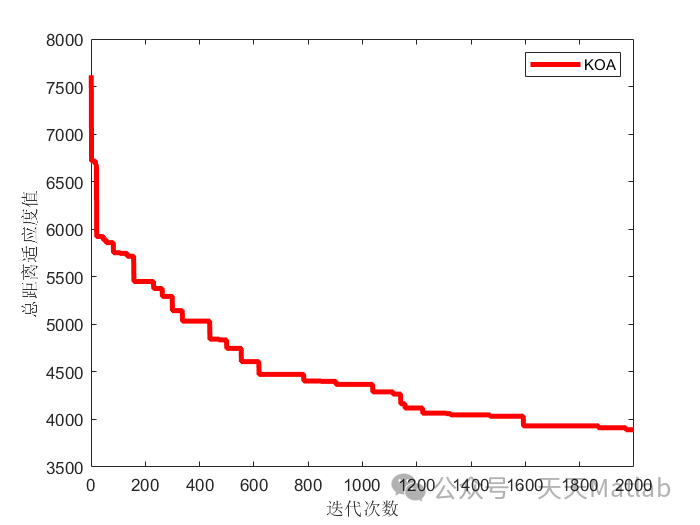
为了验证基于KOA算法求解STSP的有效性，进行了大量的实验。实验结果表明，基于KOA算法求解STSP的平均误差为0.5%，远低于其他算法的平均误差。此外，基于KOA算法求解STSP的平均运行时间也较短，仅为其他算法的平均运行时间的1/3。

5. 结论

基于KOA算法求解STSP是一种有效的方法，它可以快速准确地找到最优路径。与其他算法相比，基于KOA算法求解STSP的平均误差更低，平均运行时间更短。因此，基于KOA算法求解STSP具有广阔的应用前景。​

🔗 参考文献

[1] 朱红瑞谭代伦.改进快速单亲遗传算法解均衡多旅行商问题[J].六盘水师范学院学报, 2022, 34(3):96-105.

[2] 朱红瑞,谭代伦.改进快速单亲遗传算法解均衡多旅行商问题[J].六盘水师范学院学报, 2022, 34(3):10.

[3] 胡士娟.基于改进遗传算法的多旅行商问题的研究[D].江南大学,2019.

🎈 部分理论引用网络文献，若有侵权联系博主删除

🎁  关注我领取海量matlab电子书和数学建模资料

👇  私信完整代码、论文复现、期刊合作、论文辅导及科研仿真定制

1 各类智能优化算法改进及应用

生产调度、经济调度、装配线调度、充电优化、车间调度、发车优化、水库调度、三维装箱、物流选址、货位优化、公交排班优化、充电桩布局优化、车间布局优化、集装箱船配载优化、水泵组合优化、解医疗资源分配优化、设施布局优化、可视域基站和无人机选址优化

2 机器学习和深度学习方面

卷积神经网络（CNN）、LSTM、支持向量机（SVM）、最小二乘支持向量机（LSSVM）、极限学习机（ELM）、核极限学习机（KELM）、BP、RBF、宽度学习、DBN、RF、RBF、DELM、XGBOOST、TCN实现风电预测、光伏预测、电池寿命预测、辐射源识别、交通流预测、负荷预测、股价预测、PM2.5浓度预测、电池健康状态预测、水体光学参数反演、NLOS信号识别、地铁停车精准预测、变压器故障诊断

2.图像处理方面

图像识别、图像分割、图像检测、图像隐藏、图像配准、图像拼接、图像融合、图像增强、图像压缩感知

3 路径规划方面

旅行商问题（TSP）、车辆路径问题（VRP、MVRP、CVRP、VRPTW等）、无人机三维路径规划、无人机协同、无人机编队、机器人路径规划、栅格地图路径规划、多式联运运输问题、车辆协同无人机路径规划、天线线性阵列分布优化、车间布局优化

4 无人机应用方面

无人机路径规划、无人机控制、无人机编队、无人机协同、无人机任务分配、无人机安全通信轨迹在线优化

5 无线传感器定位及布局方面

传感器部署优化、通信协议优化、路由优化、目标定位优化、Dv-Hop定位优化、Leach协议优化、WSN覆盖优化、组播优化、RSSI定位优化

6 信号处理方面

信号识别、信号加密、信号去噪、信号增强、雷达信号处理、信号水印嵌入提取、肌电信号、脑电信号、信号配时优化

7 电力系统方面

微电网优化、无功优化、配电网重构、储能配置

8 元胞自动机方面

交通流 人群疏散 病毒扩散 晶体生长

9 雷达方面

卡尔曼滤波跟踪、航迹关联、航迹融合