递归最小二乘估计 （Recursive Least Square Estimation）

数据生成

首先生造一个例子：
$$Y=XW+v,v\sim N(0,\sigma )$$$v$ 为测量误差， 服从高斯分布。

$X$ 为已知输入， $Y$ 为已知输出，$W$ 是我们要求的。

import numpy as np

measurement_noise = 0.01

X = np.random.random((1000, 3))
W = np.random.random((3,4))
Y = X @ W
Y = Y + np.random.randn(Y.shape[0],Y.shape[1]) * measurement_noise

很简单嘛！！

最小二乘法

$$W=X^{†}Y=(X^{\top }X{)}^{-1}{X}^{\top }Y$$

w_ols = np.linalg.inv(X.T @ X) @ X.T @ Y
print('mean square error: ',mse(w_ols ,W))
print('original:\n',W)
print('estimated:\n',w_ols )
'''
mean square error:  6.212697354226623e-07
original:
 [[0.00520655 0.84260375 0.25533951 0.06882899]
 [0.28081029 0.09782934 0.26444568 0.40990159]
 [0.72283722 0.10070551 0.78082754 0.29481766]]
estimated:
 [[0.00345681 0.84162527 0.25500154 0.06916317]
 [0.28096428 0.09860053 0.26477512 0.40952032]
 [0.72422094 0.10132278 0.78102246 0.29488311]]
 '''

岭回归

$$W=(X^{\top }X+\beta I{)}^{-1}{X}^{\top }Y$$

beta = 1e-6
w_ridge = np.linalg.inv(X.T @ X + beta*np.eye(3)) @ X.T @ Y
print('mean square error: ',mse(w_ridge,W))
print('original:\n',W)
print('estimated:\n',w_ridge)
'''
mean square error:  6.212691228382955e-07
original:
[[0.00520655 0.84260375 0.25533951 0.06882899]
[0.28081029 0.09782934 0.26444568 0.40990159]
[0.72283722 0.10070551 0.78082754 0.29481766]]
estimated:
[[0.00345681 0.84162526 0.25500154 0.06916317]
[0.28096428 0.09860053 0.26477512 0.40952032]
[0.72422094 0.10132278 0.78102245 0.29488311]]
'''

递归最小二乘

initial_uncertainty = 1000

I = np.eye(X.shape[1])
P = [I * initial_uncertainty] * Y.shape[1]
w_rls = np.random.random((X.shape[1], Y.shape[1]))
R = [np.array([[measurement_noise]])] * Y.shape[1]
K = [None] * Y.shape[1]

MSE = []
for i in range(len(X)):
    H = X[i:i+1,:]
    y = Y[i:i+1,:]
    for j in range(Y.shape[1]):
        K[j] = P[j] @ H.T @ np.linalg.inv(H @ P[j] @ H.T + R[j])
        w_rls[:,j:j+1] = w_rls[:,j:j+1] + K[j] @ (y[:,j] - H @ w_rls[:,j:j+1])
        P[j] = (I - K[j] @ H) @ P[j]
    MSE.append(mse(W,w_rls))
print(w_rls)
'''
[[0.00345682 0.84162517 0.25500154 0.0691632 ]
 [0.28096434 0.09860054 0.26477521 0.4095203 ]
 [0.72422087 0.10132287 0.78102237 0.29488312]]
'''


import matplotlib.pyplot as plt
%matplotlib inline
fig, ax = plt.subplots()
ax.set_xscale("log")
ax.set_yscale("log")
ax.set_adjustable("datalim")
ax.grid()
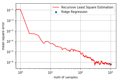
plt.ylabel('mean square error')
plt.xlabel('num of samples')
plt.plot(MSE, 'r', label='Recursive Least Square Estimation')
plt.scatter(len(X), mse(W, w_ridge), label='Ridge Regression')
plt.legend()