神经网络模型数字推理预测

MNIST数据集

MNIST是机器学习领域 最有名的数据集之一，被应用于从简单的实验到发表的论文研究等各种场合。 实际上，在阅读图像识别或机器学习的论文时，MNIST数据集经常作为实验用的数据出现。

MNIST数据集是由0到9的数字图像构成的。训练图像有6万张， 测试图像有1万张，这些图像可以用于学习和推理。MNIST数据集的一般使用方法是，先用训练图像进行学习，再用学习到的模型度量能在多大程度上对测试图像进行正确的分类。

MNIST的图像数据是28像素 × 28像素的灰度图像（1通道），各个像素的取值在0到255之间。每个图像数据都相应地标有"7" "2" "1"等标签。

使用如下脚本可以下载数据集

# coding: utf-8
try:
    import urllib.request
except ImportError:
    raise ImportError('You should use Python 3.x')
import os.path
import gzip
import pickle
import os
import numpy as np


url_base = 'http://yann.lecun.com/exdb/mnist/'
key_file = {
    'train_img':'train-images-idx3-ubyte.gz',
    'train_label':'train-labels-idx1-ubyte.gz',
    'test_img':'t10k-images-idx3-ubyte.gz',
    'test_label':'t10k-labels-idx1-ubyte.gz'
}

dataset_dir = os.path.dirname(os.path.abspath(__file__))
save_file = dataset_dir + "/mnist.pkl"

train_num = 60000
test_num = 10000
img_dim = (1, 28, 28)
img_size = 784


def _download(file_name):
    file_path = dataset_dir + "/" + file_name
    
    if os.path.exists(file_path):
        return

    print("Downloading " + file_name + " ... ")
    urllib.request.urlretrieve(url_base + file_name, file_path)
    print("Done")
    
def download_mnist():
    for v in key_file.values():
       _download(v)
        
def _load_label(file_name):
    file_path = dataset_dir + "/" + file_name
    
    print("Converting " + file_name + " to NumPy Array ...")
    with gzip.open(file_path, 'rb') as f:
            labels = np.frombuffer(f.read(), np.uint8, offset=8)
    print("Done")
    
    return labels

def _load_img(file_name):
    file_path = dataset_dir + "/" + file_name
    
    print("Converting " + file_name + " to NumPy Array ...")    
    with gzip.open(file_path, 'rb') as f:
            data = np.frombuffer(f.read(), np.uint8, offset=16)
    data = data.reshape(-1, img_size)
    print("Done")
    
    return data
    
def _convert_numpy():
    dataset = {}
    dataset['train_img'] =  _load_img(key_file['train_img'])
    dataset['train_label'] = _load_label(key_file['train_label'])    
    dataset['test_img'] = _load_img(key_file['test_img'])
    dataset['test_label'] = _load_label(key_file['test_label'])
    
    return dataset

def init_mnist():
    download_mnist()
    dataset = _convert_numpy()
    print("Creating pickle file ...")
    with open(save_file, 'wb') as f:
        pickle.dump(dataset, f, -1)
    print("Done!")

def _change_one_hot_label(X):
    T = np.zeros((X.size, 10))
    for idx, row in enumerate(T):
        row[X[idx]] = 1
        
    return T
    

def load_mnist(normalize=True, flatten=True, one_hot_label=False):
    """读入MNIST数据集
    
    Parameters
    ----------
    normalize : 将图像的像素值正规化为0.0~1.0
    one_hot_label : 
        one_hot_label为True的情况下，标签作为one-hot数组返回
        one-hot数组是指[0,0,1,0,0,0,0,0,0,0]这样的数组
    flatten : 是否将图像展开为一维数组
    
    Returns
    -------
    (训练图像, 训练标签), (测试图像, 测试标签)
    """
    if not os.path.exists(save_file):
        init_mnist()
        
    with open(save_file, 'rb') as f:
        dataset = pickle.load(f)
    
    if normalize:
        for key in ('train_img', 'test_img'):
            dataset[key] = dataset[key].astype(np.float32)
            dataset[key] /= 255.0
            
    if one_hot_label:
        dataset['train_label'] = _change_one_hot_label(dataset['train_label'])
        dataset['test_label'] = _change_one_hot_label(dataset['test_label'])
    
    if not flatten:
         for key in ('train_img', 'test_img'):
            dataset[key] = dataset[key].reshape(-1, 1, 28, 28)

    return (dataset['train_img'], dataset['train_label']), (dataset['test_img'], dataset['test_label']) 


if __name__ == '__main__':
    init_mnist()

load_mnist函数以"(训练图像 ,训练标签 )，(测试图像，测试标签 )"的多元组形式返回读入的MNIST数据。

load_mnist(normalize=True, flatten=True, one_hot_label=False) 这 样，设 置 3 个 参 数。
第 1 个参数normalize设置是否将输入图像正规化为0.0～1.0的值。如果将该参数设置为False，则输入图像的像素会保持原来的0～255。
第2个参数flatten设置是否展开输入图像（变成一维数组）。如果将该参数设置为False，则输入图像为1 × 28 × 28的三维数组；若设置为True，则输入图像会保存为由784个元素构成的一维数组。
第3个参数one_hot_label设置是否将标签保存为one-hot表示（one-hot representation）。one-hot表示是仅正确解标签为1，其余皆为0的数组，就像[0,0,1,0,0,0,0,0,0,0]这样。当one_hot_label为False时，只是像7、2这样简单保存正确解标签；当one_hot_label为True时，标签则 保存为one-hot表示。

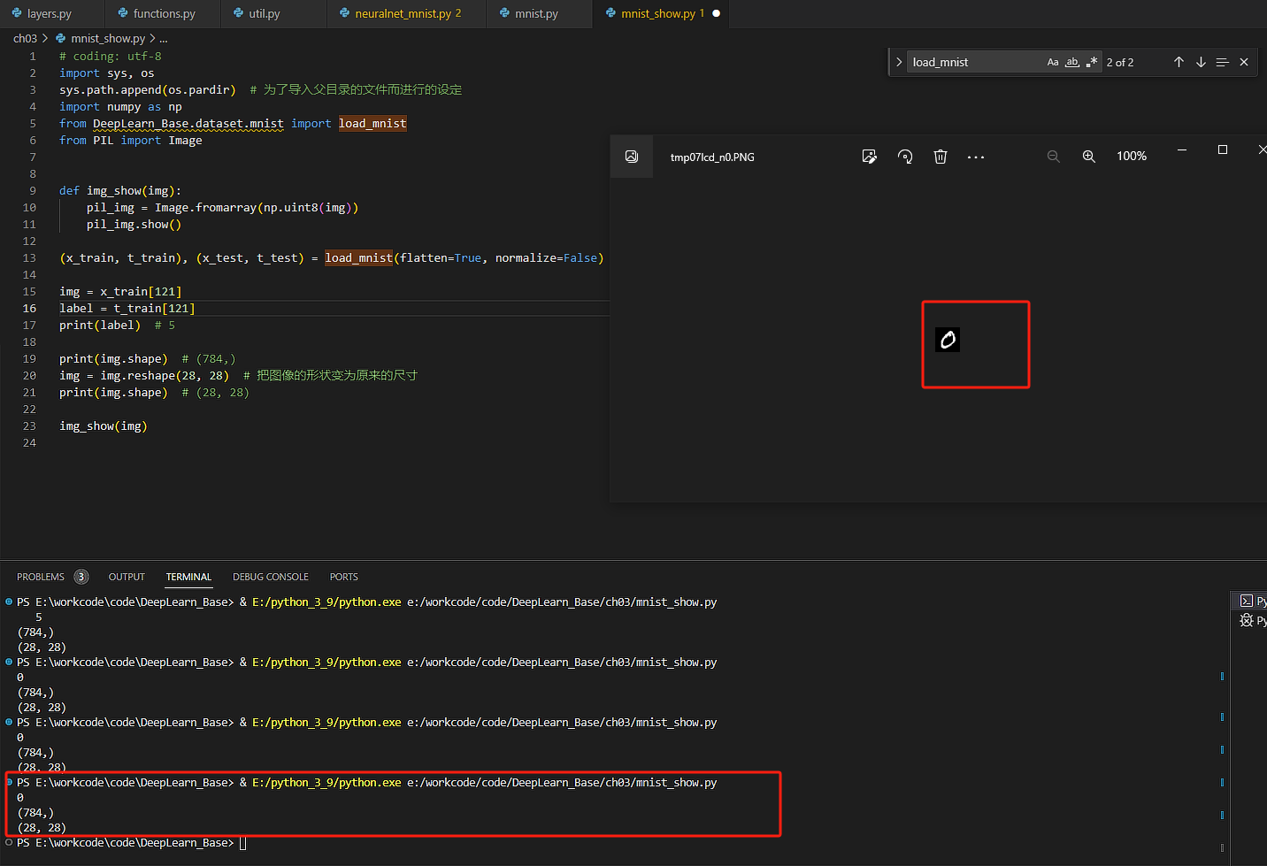
可以通过如下代码读出下载的图片

# coding: utf-8
import sys, os
sys.path.append(os.pardir)  # 为了导入父目录的文件而进行的设定
import numpy as np
from DeepLearn_Base.dataset.mnist import load_mnist
from PIL import Image


def img_show(img):
    pil_img = Image.fromarray(np.uint8(img))
    pil_img.show()

(x_train, t_train), (x_test, t_test) = load_mnist(flatten=True, normalize=False)

img = x_train[1]
label = t_train[1]
print(label)  # 5

print(img.shape)  # (784,)
img = img.reshape(28, 28)  # 把图像的形状变为原来的尺寸
print(img.shape)  # (28, 28)

img_show(img)

读出来的数据如下所示:

神经网络的推理

现在使用python的numpy结合神经网络的算法来推理图片的内容。整个流程其实就是两个部分：数据集准备、权重与偏置超参数准备。

数据集准备

使用如下代码块下载准备测试数据集:

def get_data():
    (x_train, t_train), (x_test, t_test) = load_mnist(normalize=True, flatten=True, one_hot_label=False)
    return x_test, t_test


# 下载mnist数据集
# 分别下载测试图像包、测试标签包、训练图像包、训练标签包
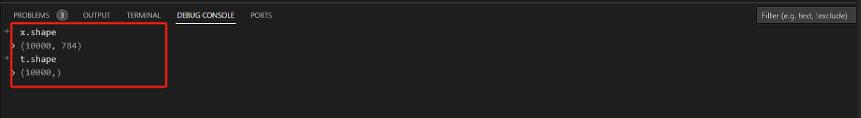
x, t = get_data()

打印输出x, t参数shape

读取实现准备好的权重参数文件pkl，同时打印出来看看其参数shape

def init_network():
    with open("E:\\workcode\\code\\DeepLearn_Base\\ch03\\sample_weight.pkl", 'rb') as f:
        network = pickle.load(f)
    return network

# 获取预训练好的权重与偏置参数
network = init_network()

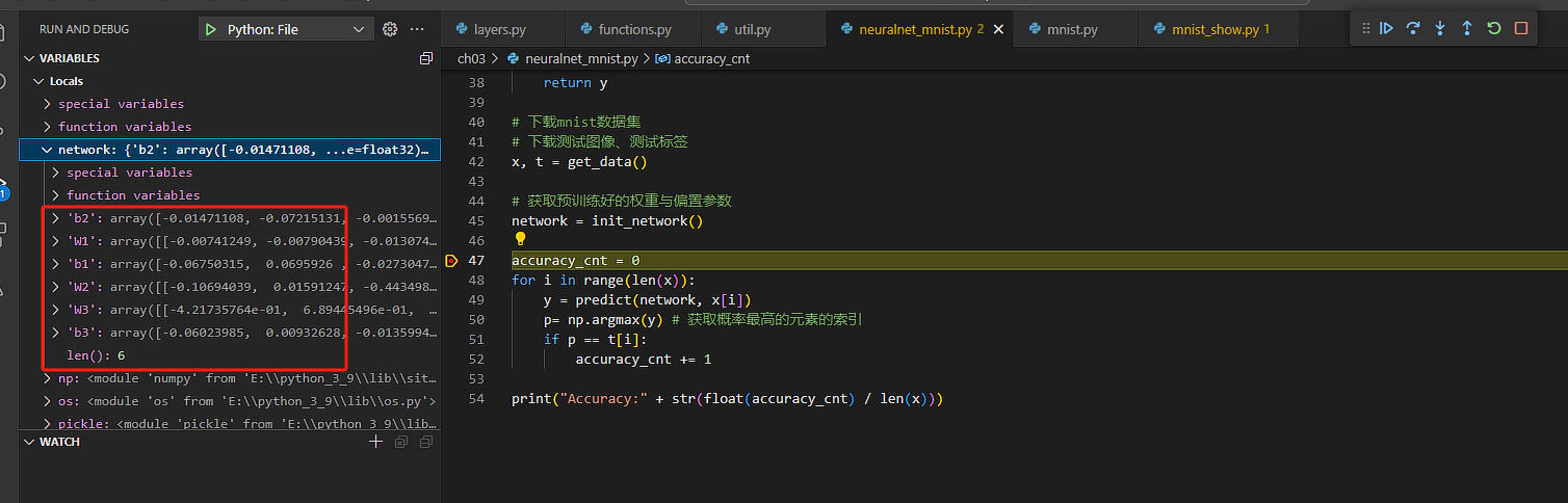
可以看到，超参数分别是3个权重参数与3个偏置参数，为了方便，稍后再打印出其shape .

超参数文件 sample_weight.pkl 是预训练好的，本文主要是从神经网络的推理角度考虑，预训练文件的准备，暂不涉及。

推理

开始执行神经网络的推理，同时打印出其各个参数的shape

def predict(network, x):
    W1, W2, W3 = network['W1'], network['W2'], network['W3']
    b1, b2, b3 = network['b1'], network['b2'], network['b3']

    # 第一层计算
    a1 = np.dot(x, W1) + b1
    z1 = sigmoid(a1)

    # 第二层计算
    a2 = np.dot(z1, W2) + b2
    z2 = sigmoid(a2)
    a3 = np.dot(z2, W3) + b3

    # 输出层
    y = softmax(a3)

    return y

accuracy_cnt = 0
for i in range(len(x)):
    y = predict(network, x[i])
    p= np.argmax(y) # 获取概率最高的元素的索引
    if p == t[i]:
        accuracy_cnt += 1

print("Accuracy:" + str(float(accuracy_cnt) / len(x)))

在predict方法中，执行了推理过程，主要是各个数学公式的计算(sigmoid,softmax,线性计算)，这些公式都是在numpy的基础上根据公式用程序语言表述出来的，具体的计算逻辑可以查阅functions.py文件。

看看各个参数的shape:

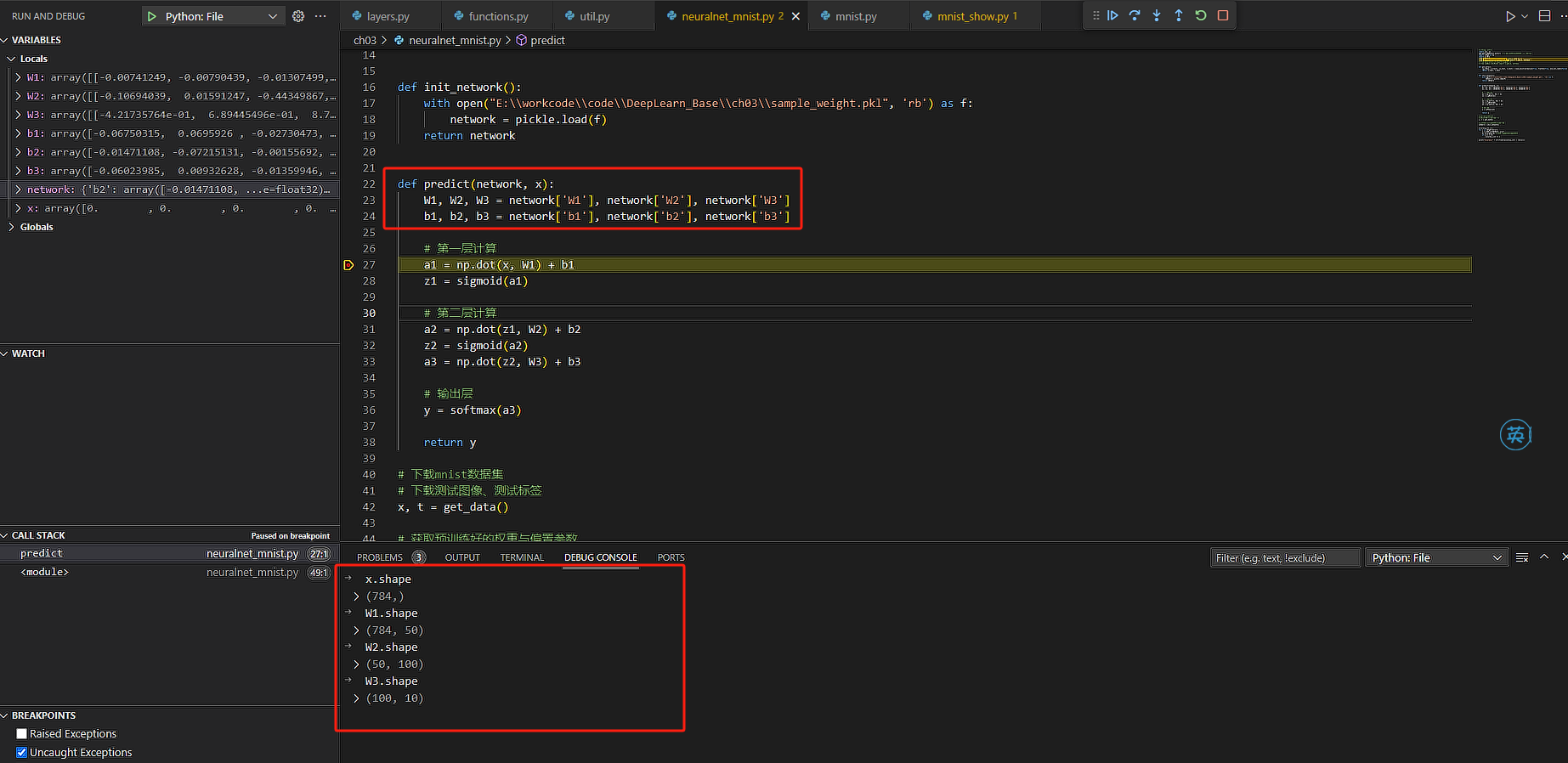
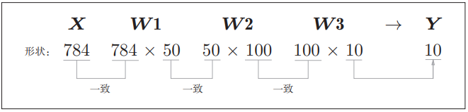
可以看看计算过程中的各个数据维度是否满足匹配: