learnopengl——Specular IBL——貌似读懂了

https://learnopengl.com/#!PBR/IBL/Specular-IBL

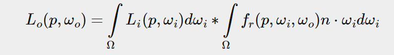
in the previous tutorial we’ve set up PBR in combination with image based lighting by pre-computing an irradiance map as the lighting’s indirect diffuse portion. In this tutorial we’ll focus on the specular part of the reflectance equation:
在上一节中，我们学习了基于图片的PBR，我们预计算了一张辐照度的图，作为光线的间接漫反射部分。本节课程，我们将重点学习反射方程中的镜面反射部分。

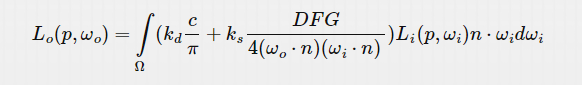
You’ll notice that the Cook-Torrance specular portion (multiplied by kS) isn’t constant over the integral and is dependent on the incoming light direction, but also the incoming view direction. Trying to solve the integral for all incoming light directions including all possible view directions is a combinatorial overload and way too expensive to calculate on a real-time basis. Epic Games proposed a solution where they were able to pre-convolute the specular part for real time purposes, given a few compromises, known as the split sum approximation.
上面的cook-torrance 模型中，对于镜面反射部分，并不是常数，它依赖于两个方向：入射光方向和视觉方向。对于所有的入射方向和所有的观察方向进行积分是不现实的。epic公式提出了一个解决这种方案，此方案叫做分布求和近似。注意是近似，真正的积分，我查了下是没有这条性质的。

the split sum approximation splits the specular part of the reflectance equation 反射方程 into two separate parts that we can individually convolute 分别进行卷积 and later combine in the PBR shader for specular indirect image based lighting. similar to how we preconvoluted the irradinace map, the split sum approximation requires an HDR environment map as its convolution input. to understand the split sum approximation we will again look at the reflectance equation, but this time only focus on the specular part (we have extracted the diffuse part in the previous tutorial):
和计算辐照度贴图一样，我们需要一个HDR模式的环境贴图，作为卷积的输入。为了能够明白分布求和近似，我们再看下这个公式。

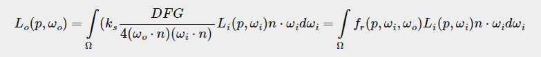
for the same (performance) reason as the irradiance convolution, we can not solve the specular part of the intergral in real time, and expect a reasonable performance. so preferably we would pre-compute this integral to get sth. like a specular IBL map, sample this map with the fragment’s normal 用片元的法线进行采样 and be done with it. however, this is where it gets a bit tricky. we were able to pre-compute the irradiance map as the integral only depend on wi 仅仅只需要光源的入射方向 and we could move the constant diffuse albedo terms out of the integral. this time, the integral depends on more than just wi as evident from the BRDF:
实时积分是不现实的，所以考虑预计算，得到一个specular IBL的贴图，然后在片段程序中，用片元的法线进行直接采样即可。
但是不像预计算辐照度贴图一样，这次的积分依赖于wi和wo，两个方向。如下面的式子可以看到：

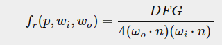
this time the integral also depends on wo and we can not really sample a pre-computed cubemap with two direction vectors. the position p is irrelevant here as described in the previous tutorial. pre-computing this integral for every possible combination of wi and wo is not practical in a real-time setting.

epic game’s split sum approximation solves the issue by splitting the pre-computation into 2 individual parts that we can later combine to get the reuslting pre-computed result we are after. the split sum approximation splits the specular integral into two separate integrals:

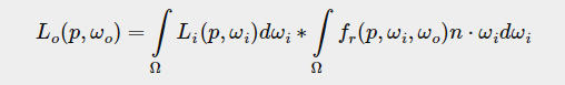
针对此，epic剔除了分布求和近似的方法。

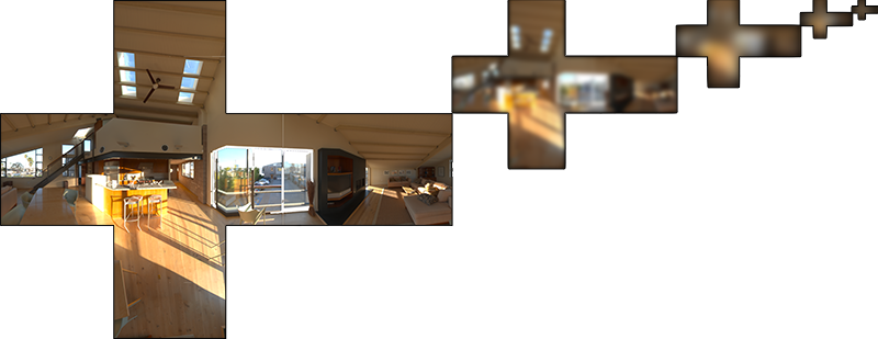
the first part (when convoluted) is known as the pre-filtered environment map which is (similar to the irradiance map) a precomputed environment convolution map, but this time taking roughness into account. for increasing roughness levels, the environment map is convoluted with more scattered 更加散落的采样向量 sample vectors, creating more blurry reflections. for each roughness level we convolute, we store the sequentially blurrier results in the pre-filtered map’s mipmap levels. for instance, a prefiltered environment map storing the pre-convoluted result of 5 different roughness in its 5 mipmap levels looks as follows:
第一个部分就是所谓的预过滤环境贴图，它其实和辐照度贴图的计算类似，也是对环境贴图进行卷积之后的结果。但是有一点区域，这次的卷积考虑的粗糙度的影响。粗糙度越高，环境贴图的卷积要使用更分散的采样向量，这样就会得到更加模糊的反射效果。对于每个粗糙度水平进行卷积，并将其有序存储在预过滤的mipmap索引内。比如下面是对5个级别的粗糙度进行卷积的结果：

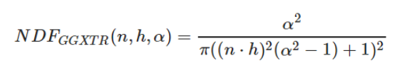
we generate the sample vectors and their scattering strength using the normal distribution function (NDF) of the cook-torrance BRDF that takes as input both a normal and view direction. as we do not know beforehand 事先 the view direction when convoluting the environment map, epic games makes a further approximation by assuming the view direction (and thus the specular reflection direction) is always equal to the output sample direction wo. this translates itself to the following code:
采样的向量和分散的程度使用的是cook-torrance BRDF中的NDF函数得到。这个函数需要两个输入量：法线和观察方向。在做卷积环境图的时候，无法提取知道观察方向，epic公司又提出了一个近似，假设观察方向恒等于反射方向wo。翻译成代码则是：

vec3 N = normalize(w_o);
vec3 R = N;
vec3 V = R;

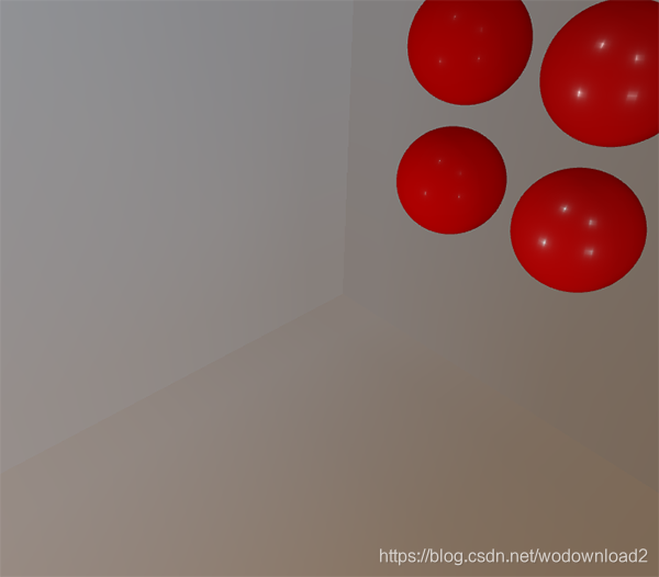
this way the pre-filtered environment convolution does not need to be aware of the view direction. this does mean we do not get nice grazing specular reflections when looking at specular surface reflections from an angle as seen in the image below
用这种方式进行的预过滤的环境卷积，不需要知道观察方向。这就意味着，如果我们不是在反射方向上进行观察的时候，则不会得到理想的反射效果。

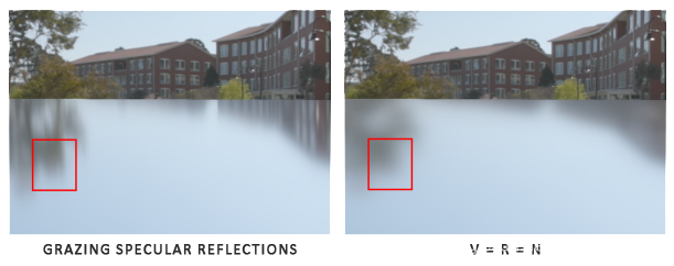
this is however generally considered a decent compromise.
但是这种折中认为是可以接受的。

the second part of the equation equals the BRDF part of the specular integral. if we pretend the incoming radiance is completely white for every direction (thus L(p,x)=1.0) we can pre-calculate the BRDF’s response given an input roughness and an input angle between the normal n and light direction wi, or n.wi. epic games stores the pre-computed BRDF’s response to each normal and light direction combination on varying roughness values in a 2D lookup texture (LUT) known as the BRDF integration map. the 2D lookup texture outputs a scale (red) and a bias value (green) to the surface’s fresnel response giving us the second part of the split specular integral:
第二个部分的是对BRDF部分进行求积分。如果我们假设入射光线的辐照度对于每个方向都是白色的，也就是说上式中的L(p,x)=1.0
那么对于给定的输入粗糙度，和一个角度（法线n和入射光方向wi的夹角）或者用n点乘wi作为输入。epic公司将每对法线和光线方向和粗糙对应的BRDF的预计算结果存储在一个2D图中。这个地方不懂。

we generate the lookup texture by treating the horizontal texture coordinate (ranged between 0.0 and 1.0) of a plane as the BRDF’s input n.wi and its vertical texture coodinate as the input roughness value. with this BRDF integration map and the pre-filtered environment map we can combine both to get the result of the specular integral:

float lod             = getMipLevelFromRoughness(roughness);
vec3 prefilteredColor = textureCubeLod(PrefilteredEnvMap, refVec, lod); //第一部分
vec2 envBRDF          = texture2D(BRDFIntegrationMap, vec2(NdotV, roughness)).xy; //第二部分
vec3 indirectSpecular = prefilteredColor * (F * envBRDF.x + envBRDF.y)  //两个部分结合

this should give u a bit of an overview on how epic game’s split sum approximation roughly approaches the indirect specular part of the reflectance equation. let us now try and build the pre-convoluted parts ourselves.

pre-filtering an HDR environment map
pre-filtering an environment map is quite similar to how we convoluted an irradiance map. 辐照度贴图 the difference being that we now account for roughness and store sequentially rougher reflections in the pre-filtered map’s mip levels.
first, we need to generate a new cubemap to hold the pre-filtered environment map data. to make sure we allocate enough memory for its mip levels we call glGenerateMipmap as an easy way to allocate the required amount of memory.
预过滤HDR环境贴图，和我们之前的卷积辐照度贴图很类似。唯一不同的是，我们要考虑到粗糙度，然后将不同程度的粗糙度贴图存储在不同的mip level的贴图中。

unsigned int prefilterMap;
glGenTextures(1, &prefilterMap);
glBindTexture(GL_TEXTURE_CUBE_MAP, prefilterMap);
for (unsigned int i = 0; i < 6; ++i)
{
    glTexImage2D(GL_TEXTURE_CUBE_MAP_POSITIVE_X + i, 0, GL_RGB16F, 128, 128, 0, GL_RGB, GL_FLOAT, nullptr);
}
glTexParameteri(GL_TEXTURE_CUBE_MAP, GL_TEXTURE_WRAP_S, GL_CLAMP_TO_EDGE);
glTexParameteri(GL_TEXTURE_CUBE_MAP, GL_TEXTURE_WRAP_T, GL_CLAMP_TO_EDGE);
glTexParameteri(GL_TEXTURE_CUBE_MAP, GL_TEXTURE_WRAP_R, GL_CLAMP_TO_EDGE);
glTexParameteri(GL_TEXTURE_CUBE_MAP, GL_TEXTURE_MIN_FILTER, GL_LINEAR_MIPMAP_LINEAR); 
glTexParameteri(GL_TEXTURE_CUBE_MAP, GL_TEXTURE_MAG_FILTER, GL_LINEAR);
glGenerateMipmap(GL_TEXTURE_CUBE_MAP);

note that because we plan to sample the prefilterMap its mipmaps u will need to make sure it minification filter is set to GL_LINEAR_MIPMAP_LINEAR to enable trilinear filtering. we store the pre-filtered specular reflections in a per-face resolution of 128 by 128 at its base mip level. this is likely to be enough for most reflections, but if u have a large number of smooth materials (think of car reflections) u may want to increase the resolution.

in the previous tutorial we convoluted the environment map by generating sample vectors uniformaly spread over the hemisphere Ω using spherical coordinates. while this works just fine for irradiance, for specular reflections it is less efficient. when it comes to specular reflections, based on the roughness of a surface, the light reflects closely or roughly around a reflection vector r over a normal n, but (unless the surface is extremely rough) around the reflection vector nonetheless:这也就是为什么在预计算镜面反射的时候，要进行重要性采样。

the general shape of possible outgoing light reflections is known as the specular lobe. 形状类似花瓣. as roughness increases, the specular lobe’s size increases; and the shape of the specular lobe changes on varying incoming light directions. the shape of the specular lobe is thus highly dependent on the material.

when it comes to the microsurface model, we can imagine the specular lobe as the reflection orientation about the microfacet halfway vectors given some incoming light direction. seeing as most light rays end up in a specular lobe reflected around the microfacet halfway vectors it makes sense to generate the sample vecors in a similar fashion as most would otherwise be wasted. this process is known as importance sampling. 重要性采样

monte carlo integration and importance sampling
to fully get a grasp of importance sampling it is relevant we first delve into the mathematical construct known as Monte Carlo intergration. Monte carlo integration revolves mostly around a combination of statistics and probability theory. monte carlo helps us in discretely solving the problem of figuring out some statistic or value of a population without having to take all of the population into consideration.

for instance, let us say u want to count the average height of all citizens of a country. to get your result, u could measure every citizen and average their height which will give u the exact answer u are looking for. however, since most countries have a considerable population this is not a realistic approach: it would take too much effort and time.
比如，要求一个国家的市民的平均身高。需要加权所有人的身高，但是一个国家的人口特别的多的时候，这个方法是不可行的。

a different approach is to pick a much smaller completely random (unbiased) subset of this population, measure their height and average the result. this population could be as small as a 100 people. while not as accurate as the exact answer, u will get an answer that is relatively close to the ground truth. this is known as the law of large numbers. 大数定律 the idea is that if u measure a smaller set of size N of truly random samples from the total population, the result will be relatively close to the true answer and gets closer as the number of samples N increases.

monte carlo integration builds on this law of large numbers and takes the same approach in solving an integral. rather than solving an integral for all possible (theoretically infinite) sample value x, simply generate N sample values randomly picked from the total population and average. as N increases we are guaranteed to get a result closer to the exact answer of the integral:

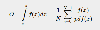
to solve the integral, we take N random samples over the population a to b, add them together and divide by the total number of samples to average them. the pdf stands for the probability density function 概率密度函数 that tells us the probability a specific sample occurs over the total sample set. for instance, the pdf of the height of a population would look a bit like this:

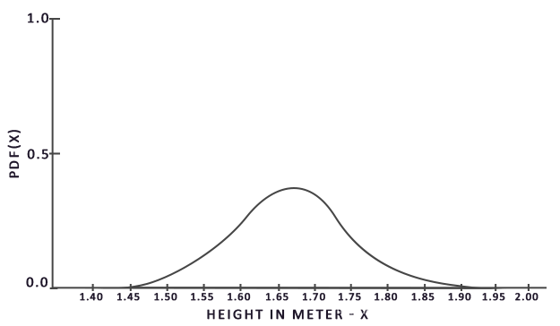
from this graph we can see that if we take any random sample of population, there is a higher chance of picking a sample of someone of height 1.70, compared to the lower probability of the sample being of height 1.50.
由图可知，如果我们采样一个随机的身高，那么采样到身高为1.70的概率应该大一点。而采样到1.50的概率要小一点。

when it comes to monte carlo integration, some samples might have a higher probability of being generated than others. this is why for any general monte carlo estimation we divide or multiply the sampled value by the sample probabiltiy according to a pdf. so far, in each of our cases of estimating an integral, the samples we have generated were uniform, having the exact same chance of being generated. our estimations so far were unbiased, meaning that given an ever-increasing amount of samples we will eventually coverage to the exact solution of the integral.
采样的值，和采样的值的概率密度函数进行除法运算，得到无偏差的加权。

however, some monte carlo estimators are biased, meaning that the generated samples are not completely random, but focused towards a specific value or direction. these biased monte carlo estimators have a faster rate of convergence meaning they can converge to the exact solution at a much faster rate, but due to their biased nature it is likely they will not ever converge to the exact solution. this is generally an acceptable tradeoff, especially in computer graphics, as the exact solution is not too important as long as the results are visually acceptable. as we will soon see with importance sampling (which uses a biased estimator) the generated samples are biased towards specific directions in which case we account for this by multiplying or dividing each sample by its cooresponding pdf.

monte carlo integration is quite prevalent in computer graphics as it is a fairly intuitive way to approximate continuous integrals in a discrete and efficient fashion: take any area/volume to sample over (like the hemisphere Ω), genereate N amount of random samples within the area/volume and sum and weigh every sample contribution to the final result.

monte carlo integration is an extensive mathematical topic and i will not delve much further into the specifics, but we will mention that there are also multiple ways of generating the random samples. by default, each sample is completely (pseudo) random as we are used to, but by utilizing certain properties of semi-random sequences we can generate sample vectors that are still random, but have interesting properties. for instance, we can do monte carlo integration on sth. called low-disrepancy sequences which still generate random samples, but each sample is more envenly distributed:

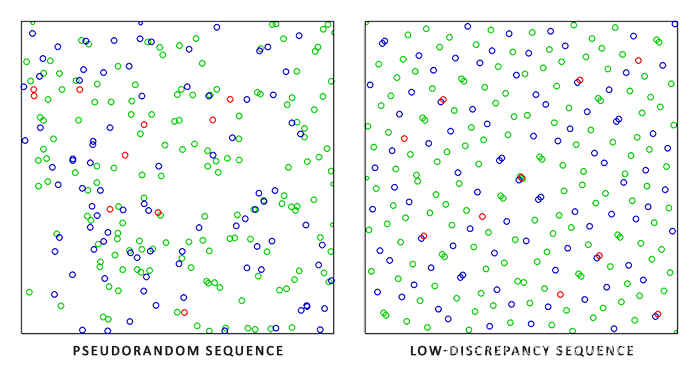
when using a low-discrepency sequence for generating the monte carlo sampel vectors, the process is known as quasi-monte carlo integration. quasi-monte carlo methods have a faster rate of convergence which makes them interesting for performance heavy applications.

given our newly obtained knowledge of monte carlo and quasi-monte carlo integration, there is an interesting property we can use for an even faster rate of convergence known as importance sampling. we have mentioned it before in this tutorial, but when it comes to specular reflections of light, the reflected light vectors are constrained in a specular lobe with its size determined by the roughness of the surface. seeing as any (quasi-) randomly generated sample outside the specular lobe is not relevant to the specular integral it makes sense to focus the sample generation to within the specular lobe, at the cost of making the monte carlo estimator biased.

this is in essence what importance sampling is about: generate sample vectors in some region constrained by the roughness oriented around the microfacet’s halfway vector. by combing quasi-monte carlo sampling with a low-disrepancy sequence and biasing the sample vectors using importance sampling we get a high rate of convergence. because we reach the solution at a faster rate, we will need less samples to reach an approximation that is sufficient enough. because of this, the combination even allows graphics applications to solve the specular integral in real-time, albeit 尽管 it still significantly slower than pre-computing the results.

a low-discrepancy sequence 低差异
in this tutorial we will pre-compute the specular portion of the indirect reflectance equation using importance sampling given a random low-discrepency sequence based on the quasi-monte carlo method. the sequence we will be using is known as the Hammersley Sequence as carefully described by Holger Dammertz. the hammersley sequence is based on the van der corpus sequence which mirros a decimal 小数 binary representation around its decimal point.

given some neat bit tricks we can quite efficiently generate the van der corpus sequence in a shader program which we will use to get a hammersley sequence sample i over N total samples:

float RadicalInverse_VdC(uint bits) 
{
    bits = (bits << 16u) | (bits >> 16u);
    bits = ((bits & 0x55555555u) << 1u) | ((bits & 0xAAAAAAAAu) >> 1u);
    bits = ((bits & 0x33333333u) << 2u) | ((bits & 0xCCCCCCCCu) >> 2u);
    bits = ((bits & 0x0F0F0F0Fu) << 4u) | ((bits & 0xF0F0F0F0u) >> 4u);
    bits = ((bits & 0x00FF00FFu) << 8u) | ((bits & 0xFF00FF00u) >> 8u);
    return float(bits) * 2.3283064365386963e-10; // / 0x100000000
}
// ----------------------------------------------------------------------------
vec2 Hammersley(uint i, uint N)
{
    return vec2(float(i)/float(N), RadicalInverse_VdC(i));
}  

ggx importance sampling
instead of uniformly or randomly (monte carlo) generating sample vectors over the integral’s hemisphere Ω we will generate sampel vectors biased towards the general reflection orientation of the microsurface halfway vector based on the surface’s roughness. the sampling process will be similar to what have seen before: begin a large loop, generate a random (low-discrepancy) sequence value, take the sequence value to generate a sample vector in tangent space, transform to world space and sample the scene’s randiance. what is different is that we now use a low-discrepancy sequence value as input to generate a sample vector:

const uint SAMPLE_COUNT = 4096u;
for(uint i = 0u; i < SAMPLE_COUNT; ++i)
{
    vec2 Xi = Hammersley(i, SAMPLE_COUNT);   

additionally, to build a sample vector, we need some way of orientating and biasing the sample vector towards the specular lobe of some surface roughness. we can take the NDF as described in the theory tutorial and combine the ggx ndf in the spherical sample vector process as described by epic games:

vec3 ImportanceSampleGGX(vec2 Xi, vec3 N, float roughness)
{
    float a = roughness*roughness;
	
    float phi = 2.0 * PI * Xi.x;
    float cosTheta = sqrt((1.0 - Xi.y) / (1.0 + (a*a - 1.0) * Xi.y));
    float sinTheta = sqrt(1.0 - cosTheta*cosTheta);
	
    // from spherical coordinates to cartesian coordinates
    vec3 H;
    H.x = cos(phi) * sinTheta;
    H.y = sin(phi) * sinTheta;
    H.z = cosTheta;
	
    // from tangent-space vector to world-space sample vector
    vec3 up        = abs(N.z) < 0.999 ? vec3(0.0, 0.0, 1.0) : vec3(1.0, 0.0, 0.0);
    vec3 tangent   = normalize(cross(up, N));
    vec3 bitangent = cross(N, tangent);
	
    vec3 sampleVec = tangent * H.x + bitangent * H.y + N * H.z;
    return normalize(sampleVec);
}

this gives us a sample vector somewhat oriented around the expected microsurface’s halfway vector based on some input roughness and the low-discrepancy sequence value xi. note that epic games uses the squared roughness for better visual results as based on disney’s original pbr research.

with the low-discrepancy hammersley sequence and sample generation defined we can finalize the pre-filter convolution shader:

#version 330 core
out vec4 FragColor;
in vec3 localPos;

uniform samplerCube environmentMap;
uniform float roughness;

const float PI = 3.14159265359;

float RadicalInverse_VdC(uint bits);
vec2 Hammersley(uint i, uint N);
vec3 ImportanceSampleGGX(vec2 Xi, vec3 N, float roughness);
  
void main()
{		
    vec3 N = normalize(localPos);    
    vec3 R = N;
    vec3 V = R;

    const uint SAMPLE_COUNT = 1024u;
    float totalWeight = 0.0;   
    vec3 prefilteredColor = vec3(0.0);     
    for(uint i = 0u; i < SAMPLE_COUNT; ++i)
    {
        vec2 Xi = Hammersley(i, SAMPLE_COUNT);
        vec3 H  = ImportanceSampleGGX(Xi, N, roughness);
        vec3 L  = normalize(2.0 * dot(V, H) * H - V);

        float NdotL = max(dot(N, L), 0.0);
        if(NdotL > 0.0)
        {
            prefilteredColor += texture(environmentMap, L).rgb * NdotL; //这里乘以NdotL是为考虑权重
            totalWeight      += NdotL;
        }
    }
    prefilteredColor = prefilteredColor / totalWeight;

    FragColor = vec4(prefilteredColor, 1.0);
}  
  

we pre-filter the enviroment, based on some input roughness that varies over each mipmap level of the pre-filter cubemap (from 0.0 to 1.0) and store the result in prefilteredColor. the resulting prefilteredColor is divided by the total sample weight, where samples with less influence on the final result (for small NdotL) contribute less to the final weight.
粗糙度的是在（0~1）范围，然后采样不同的等级的cubemap图。

capturing pre-filter mipmap levels
what is left to do is let opengl pre-filter the environment map with different roughness values over multiple mipmap levels .this is actually fairly easy to do with the original setup of the irradiance tutorial:

prefilterShader.use();
prefilterShader.setInt("environmentMap", 0);
prefilterShader.setMat4("projection", captureProjection);
glActiveTexture(GL_TEXTURE0);
glBindTexture(GL_TEXTURE_CUBE_MAP, envCubemap);

glBindFramebuffer(GL_FRAMEBUFFER, captureFBO);
unsigned int maxMipLevels = 5;
for (unsigned int mip = 0; mip < maxMipLevels; ++mip)
{
    // reisze framebuffer according to mip-level size.
    unsigned int mipWidth  = 128 * std::pow(0.5, mip);
    unsigned int mipHeight = 128 * std::pow(0.5, mip);
    glBindRenderbuffer(GL_RENDERBUFFER, captureRBO);
    glRenderbufferStorage(GL_RENDERBUFFER, GL_DEPTH_COMPONENT24, mipWidth, mipHeight);
    glViewport(0, 0, mipWidth, mipHeight);

    float roughness = (float)mip / (float)(maxMipLevels - 1);
    prefilterShader.setFloat("roughness", roughness);
    for (unsigned int i = 0; i < 6; ++i)
    {
        prefilterShader.setMat4("view", captureViews[i]);
        glFramebufferTexture2D(GL_FRAMEBUFFER, GL_COLOR_ATTACHMENT0, 
                               GL_TEXTURE_CUBE_MAP_POSITIVE_X + i, prefilterMap, mip);

        glClear(GL_COLOR_BUFFER_BIT | GL_DEPTH_BUFFER_BIT);
        renderCube();
    }
}
glBindFramebuffer(GL_FRAMEBUFFER, 0);   

the process is similar to the irradiance map convolution, but this time we scale the framebuffer’s dimensions to the appropriate mipmap scale, each mip level reducing the dimensions by 2. additionaly, we specify the mip level we are rendering into in glFramebufferTexture2D’s last parameter and pass the roughness we are pre-filtering for to the pre-filter shader.

this should give us a properly pre-filtered environment map that returns blurrier reflections the higher mip level we access it from . if we display the pre-filtered environment cubemap in the skybox shader and forecefully sample somewhat above its first mip level in its shader like so:

vec3 envColor = textureLod(environmentMap, WorldPos, 1.2).rgb; 

We get a result that indeed looks like a blurrier version of the original environment: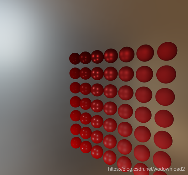

If it looks somewhat similar you’ve successfully pre-filtered the HDR environment map. Play around with different mipmap levels to see the pre-filter map gradually change from sharp to blurry reflections on increasing mip levels.

pre-filter convolution artifacts
while the current pre-filter map works fine for most purposes, sooner or later u will come across several render artifacts that are directly related to the pre-filter convolution. i will list the most common here including how to fix them.

会遇到一些合成的错误。

cube map seams at high roughness
sampling the pre-filter map on surfaces with a rough surface means sampling the pre-filter map on some of its lower mip levels. when sampling cubemaps, opengl by default does not linearly interpolate acoss cubemap faces. because the lower mip levels are both of a lower resolution and the pre-filter map is convoluted with a much larger sample code, the lack of between-cube-face filtering becomes quite apparent:

luckily for us, opengl gives us the option to propertly filter across cubemap faces by enabling GL_TEXTURE_CUBE_MAP_SEAMLESS:

glEnable(GL_TEXTURE_CUBE_MAP_SEAMLESS);

simply enable this property somewhere at the start of your application and the seams will be gone. 分割线

bright dots in the pre-filter convolution
due to high frequency details and wildly varying light intensities in specular reflections, convoluting the specular reflections requires a large number of samples to properly account for the wildly varying nature of HDR environmental reflections. we already take a very large number of samples, but on some environments it might still not be enough at some of the rougher mip levels in which case u will start seeing dotted patterns emerge around the bright areas:

one option is to further increase the sample count, but this will not be enough for all environments. as described by chetan jags https://chetanjags.wordpress.com/2015/08/26/image-based-lighting/
we can reduce this artifact by (during the pre-filter convolution) not directly sampling the environment map, but sampling a mip level of the environment map based on the integral’s PDF and the roughness:

float D   = DistributionGGX(NdotH, roughness);
float pdf = (D * NdotH / (4.0 * HdotV)) + 0.0001; 

float resolution = 512.0; // resolution of source cubemap (per face)
float saTexel  = 4.0 * PI / (6.0 * resolution * resolution);
float saSample = 1.0 / (float(SAMPLE_COUNT) * pdf + 0.0001);

float mipLevel = roughness == 0.0 ? 0.0 : 0.5 * log2(saSample / saTexel); 

do not forget to enable trilinear filtering on the environment map u want to sample its mip levels from:

glBindTexture(GL_TEXTURE_CUBE_MAP, envCubemap);
glTexParameteri(GL_TEXTURE_CUBE_MAP, GL_TEXTURE_MIN_FILTER, GL_LINEAR_MIPMAP_LINEAR); 

and let opengl generate the mipmaps after the cubemap’s base texture is set:

// convert HDR equirectangular environment map to cubemap equivalent
[...]
// then generate mipmaps
glBindTexture(GL_TEXTURE_CUBE_MAP, envCubemap);
glGenerateMipmap(GL_TEXTURE_CUBE_MAP);

this works surprisingly well and should remove most, if no all, dots in your pre-filter map on rougher surfaces.

pre-computing the BRDF
with the pre-filtered environment up and running, we can focus on the second part of the split-sum approximation: the BRDF.

let us briefly review the specular split sum approximation again:

we have pre-computed the left part of the split sum approximation in the pre-filter map over different roughness levels. the right side requires us to convolute the BRDF equation over the angle n.wo, the surface roughness and fresnel’s F0. this is similar to integrating the specular BRDF with a solid-white environment or a constant radiance Li of 1.0. convoluting the BRDF over 3 variables is a bit much, but we can move F0 out of the specular BRDF equation:

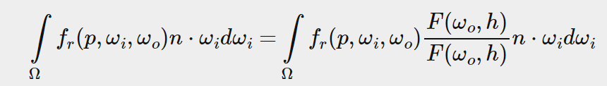
With F being the Fresnel equation. Moving the Fresnel denominator 分母 to the BRDF gives us the following equivalent equation:

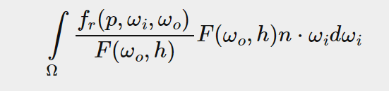
substituting the right-most F with the Fresnel-Schlick approximation gives us:

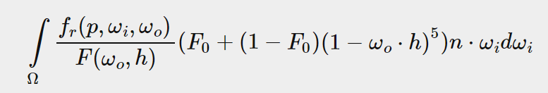
let us replace (1−ωo⋅h)^5 by α to make it easier to solve for F0:

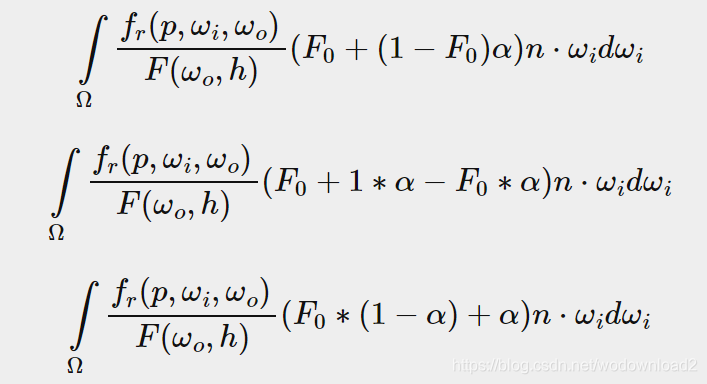
then we split the fresnel function F over two integrasl:

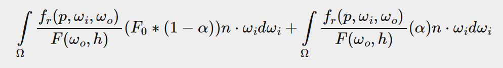
This way, F0 is constant over the integral and we can take F0 out of the integral. Next, we substitute α back to its original form giving us the final split sum BRDF equation:

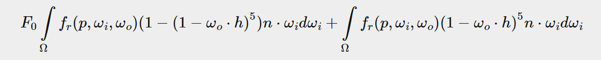
the two resulting intergrals represent a scale and a bias to F0 respectively. note that as f(p,ωi,ωo) already contains a term for F they both cancel out, removing F from f.？？？

in a similar fashion to the earlier covoluted environment maps, we can convolute the BRDF equations on their inputs: the angle between n and wo and the roughness, and store the convoluted result in a texture. we store the convoluted results in a 2D lookup texture (LUT) known as a BRDF intergration map that we later use in our PBR lighting shader to get the final convoluted indirect specular result.

the BRDF convolution shader operates on a 2D plane, using its 2D texture coordinates directly as inputs to the BRDF convolution (NdotV and roughness 咦？他们的值在0到1之间). the convolution code is largely similar to the pre-filter convolution, except that it now process the sample vector according to our BRDF’s geometry function and fresnel-schlick’s approximation:

vec2 IntegrateBRDF(float NdotV, float roughness)
{
    vec3 V;
    V.x = sqrt(1.0 - NdotV*NdotV);
    V.y = 0.0;
    V.z = NdotV;

    float A = 0.0;
    float B = 0.0;

    vec3 N = vec3(0.0, 0.0, 1.0);

    const uint SAMPLE_COUNT = 1024u;
    for(uint i = 0u; i < SAMPLE_COUNT; ++i)
    {
        vec2 Xi = Hammersley(i, SAMPLE_COUNT);
        vec3 H  = ImportanceSampleGGX(Xi, N, roughness);
        vec3 L  = normalize(2.0 * dot(V, H) * H - V);

        float NdotL = max(L.z, 0.0);
        float NdotH = max(H.z, 0.0);
        float VdotH = max(dot(V, H), 0.0);

        if(NdotL > 0.0)
        {
            float G = GeometrySmith(N, V, L, roughness);
            float G_Vis = (G * VdotH) / (NdotH * NdotV);
            float Fc = pow(1.0 - VdotH, 5.0);

            A += (1.0 - Fc) * G_Vis;
            B += Fc * G_Vis;
        }
    }
    A /= float(SAMPLE_COUNT);
    B /= float(SAMPLE_COUNT);
    return vec2(A, B);
}
// ----------------------------------------------------------------------------
void main() 
{
    vec2 integratedBRDF = IntegrateBRDF(TexCoords.x, TexCoords.y);
    FragColor = integratedBRDF;
}

as u can see the BRDF convolution is a direct translation from the mathematics to code. we take both the angle θ and the roughness as input, generate a sample vector with importance sampling, process it over the geometry and the derived fresnel term of the BRDF, and output both a scale and a bias to to F0 for each sample, averaging them in the end.

u might have recalled from the theory tutorial that the geometry term of the BRDF is silightly different when used alongside IBL as its k variable has a slightly different interpretation:

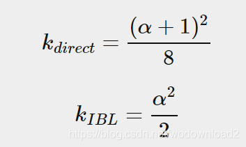
since the BRDF convolution is part of the specular IBL integral we will use KIBL for the Schlick-GGX geometry function:

float GeometrySchlickGGX(float NdotV, float roughness)
{
    float a = roughness;
    float k = (a * a) / 2.0;

    float nom   = NdotV;
    float denom = NdotV * (1.0 - k) + k;

    return nom / denom;
}
// ----------------------------------------------------------------------------
float GeometrySmith(vec3 N, vec3 V, vec3 L, float roughness)
{
    float NdotV = max(dot(N, V), 0.0);
    float NdotL = max(dot(N, L), 0.0);
    float ggx2 = GeometrySchlickGGX(NdotV, roughness);
    float ggx1 = GeometrySchlickGGX(NdotL, roughness);

    return ggx1 * ggx2;
}  

note that while k takes a as its parameter we did not square roughness as a as we originally did for other interpretations of a; likely as a is squared here already. i am not sure whether this is an inconsistency on epic game’s part or the original disney paper, but directly translating roughness to a gives the BRDF integration map that is identical to epic game’s version.

finally, to store the BRDF convolution result we will generate a 2D texture of a 512 by 512 resolution.

unsigned int brdfLUTTexture;
glGenTextures(1, &brdfLUTTexture);

// pre-allocate enough memory for the LUT texture.
glBindTexture(GL_TEXTURE_2D, brdfLUTTexture);
glTexImage2D(GL_TEXTURE_2D, 0, GL_RG16F, 512, 512, 0, GL_RG, GL_FLOAT, 0);
glTexParameteri(GL_TEXTURE_2D, GL_TEXTURE_WRAP_S, GL_CLAMP_TO_EDGE);
glTexParameteri(GL_TEXTURE_2D, GL_TEXTURE_WRAP_T, GL_CLAMP_TO_EDGE);
glTexParameteri(GL_TEXTURE_2D, GL_TEXTURE_MIN_FILTER, GL_LINEAR);
glTexParameteri(GL_TEXTURE_2D, GL_TEXTURE_MAG_FILTER, GL_LINEAR);

note that we use a 16-bit precision floating format as recommended by epic games. be sure to set the wrapping mode to GL_CLAMP_TO_EDGE to prevent edge sampling artifacts.

then, we re-use the same framebuffer object and run this shader over an NDC screen-space quad:

glBindFramebuffer(GL_FRAMEBUFFER, captureFBO);
glBindRenderbuffer(GL_RENDERBUFFER, captureRBO);
glRenderbufferStorage(GL_RENDERBUFFER, GL_DEPTH_COMPONENT24, 512, 512);
glFramebufferTexture2D(GL_FRAMEBUFFER, GL_COLOR_ATTACHMENT0, GL_TEXTURE_2D, brdfLUTTexture, 0);

glViewport(0, 0, 512, 512);
brdfShader.use();
glClear(GL_COLOR_BUFFER_BIT | GL_DEPTH_BUFFER_BIT);
RenderQuad();

glBindFramebuffer(GL_FRAMEBUFFER, 0); 

The convoluted BRDF part of the split sum integral should give you the following result:

with both the pre-filtered environment map and the BRDF 2D LUT we can re-construct the indirect specular integral according to the split sum approximation. the combined result then acts as the indirect or ambient specular light.

completing the IBL reflectance
to get the indirect specular part of the reflectance equation up and running we need to stitch both parts of 缝合？ the split sum approximation together. let us start by adding the pre-computed lighting data to the top of our PBR shader:

uniform samplerCube prefilterMap;
uniform sampler2D   brdfLUT;  

first, we get the indirect specular reflections of the surface by sampling the pre-filtered environment map using the reflection vector. note that we sample the appropriate mip level based on the surface roughness, giving rougher surfaces blurrier specular reflections.

void main()
{
    [...]
    vec3 R = reflect(-V, N);   

    const float MAX_REFLECTION_LOD = 4.0;
    vec3 prefilteredColor = textureLod(prefilterMap, R,  roughness * MAX_REFLECTION_LOD).rgb;    
    [...]
}

in the pre-filter step we only convoluted the environment map up to a maximum of 5 mip levels (0 to 4), which we denote here as MAX_REFLECTION_LOD to ensure we do not sample a mip level where there is no (relevant) data.

Then we sample from the BRDF lookup texture given the material’s roughness and the angle between the normal and view vector:

vec3 F        = FresnelSchlickRoughness(max(dot(N, V), 0.0), F0, roughness);
vec2 envBRDF  = texture(brdfLUT, vec2(max(dot(N, V), 0.0), roughness)).rg;
vec3 specular = prefilteredColor * (F * envBRDF.x + envBRDF.y);

Given the scale and bias to F0 (here we’re directly using the indirect Fresnel result F) from the BRDF lookup texture we combine this with the left pre-filter portion of the IBL reflectance equation and re-construct the approximated integral result as specular.

this gives us the indirect specular part of the reflectance equation. now, combine this with the diffuse part of reflectance equation from the last tutorial and we get the full PBR IBL result:

vec3 F = FresnelSchlickRoughness(max(dot(N, V), 0.0), F0, roughness);
vec3 kS = F;
vec3 kD = 1.0 - kS;
kD *= 1.0 - metallic;	  
  
vec3 irradiance = texture(irradianceMap, N).rgb;
vec3 diffuse    = irradiance * albedo;
  
const float MAX_REFLECTION_LOD = 4.0;
vec3 prefilteredColor = textureLod(prefilterMap, R,  roughness * MAX_REFLECTION_LOD).rgb;   
vec2 envBRDF  = texture(brdfLUT, vec2(max(dot(N, V), 0.0), roughness)).rg;
vec3 specular = prefilteredColor * (F * envBRDF.x + envBRDF.y);
  
vec3 ambient = (kD * diffuse + specular) * ao; 

Note that we don’t multiply specular by kS as we already have a Fresnel multiplication in there.

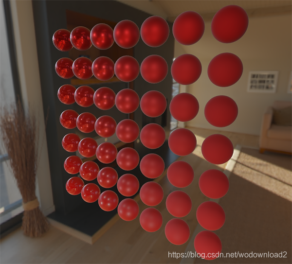
Now, running this exact code on the series of spheres that differ by their roughness and metallic properties we finally get to see their true colors in the final PBR renderer:

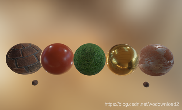
We could even go wild, and use some cool textured PBR materials:

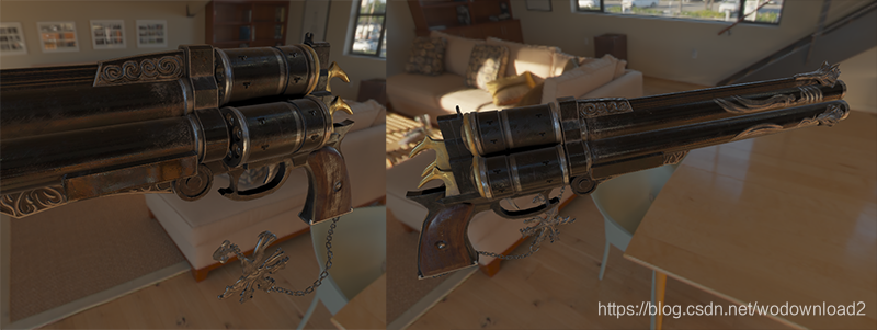
Or load this awesome free PBR 3D model by Andrew Maximov:

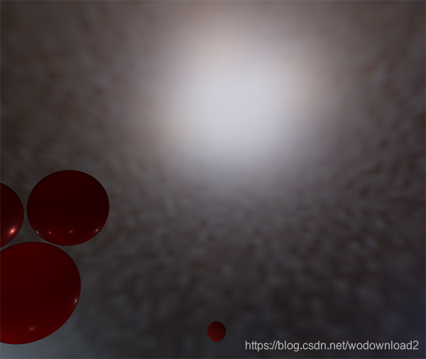
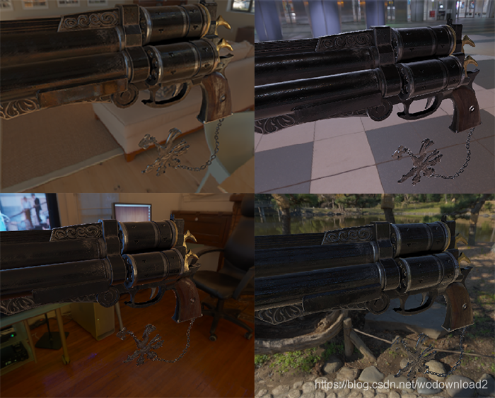
I’m sure we can all agree that our lighting now looks a lot more convincing 看起来让人更加的信服了. What’s even better, is that our lighting looks physically correct 不管我们用哪张环境贴图，看起来更加物理正确了, regardless of which environment map we use. Below you’ll see several different pre-computed HDR maps, completely changing the lighting dynamics, but still looking physically correct without changing a single lighting variable!

well, this PBR adventure turned out to be quite a long journey. there a lot of steps and thus a lot that could go wrong so carefully work your way through the sphere scene or textured scene code samples (including all shaders) if u are stuck, or check and ask around in the comments.

下面贴图原文中提供的，几个用到的shader的完整代码：

1、预过滤的环境贴图：pre-filtered environment map
由于代码比较多，我们就将直接代码中添加分析注释了。

#version 330 core
out vec4 FragColor;
in vec3 WorldPos;

uniform samplerCube environmentMap; //C++代码传入的一张图
uniform float roughness; //粗糙度，也是外部传入

const float PI = 3.14159265359;
// ----------------------------------------------------------------------------
// GGX函数，几何遮蔽函数，传入的参数偶，宏观法线，半角向量，粗糙度，这里使用最常用的GGX法线分布函数，其公式为：
![在这里插入图片描述](https://img-blog.csdnimg.cn/20191118144031350.png)
float DistributionGGX(vec3 N, vec3 H, float roughness)
{
    float a = roughness*roughness;
    float a2 = a*a;
    float NdotH = max(dot(N, H), 0.0);
    float NdotH2 = NdotH*NdotH;

    float nom   = a2;
    float denom = (NdotH2 * (a2 - 1.0) + 1.0);
    denom = PI * denom * denom;

    return nom / denom;
}
// ----------------------------------------------------------------------------
// http://holger.dammertz.org/stuff/notes_HammersleyOnHemisphere.html
// efficient VanDerCorpus calculation.
float RadicalInverse_VdC(uint bits) 
{
     bits = (bits << 16u) | (bits >> 16u);
     bits = ((bits & 0x55555555u) << 1u) | ((bits & 0xAAAAAAAAu) >> 1u);
     bits = ((bits & 0x33333333u) << 2u) | ((bits & 0xCCCCCCCCu) >> 2u);
     bits = ((bits & 0x0F0F0F0Fu) << 4u) | ((bits & 0xF0F0F0F0u) >> 4u);
     bits = ((bits & 0x00FF00FFu) << 8u) | ((bits & 0xFF00FF00u) >> 8u);
     return float(bits) * 2.3283064365386963e-10; // / 0x100000000
}
// ----------------------------------------------------------------------------
vec2 Hammersley(uint i, uint N)
{
	return vec2(float(i)/float(N), RadicalInverse_VdC(i));
}
// ----------------------------------------------------------------------------
vec3 ImportanceSampleGGX(vec2 Xi, vec3 N, float roughness)
{
	float a = roughness*roughness;
	
	float phi = 2.0 * PI * Xi.x;
	float cosTheta = sqrt((1.0 - Xi.y) / (1.0 + (a*a - 1.0) * Xi.y));
	float sinTheta = sqrt(1.0 - cosTheta*cosTheta);
	
	// from spherical coordinates to cartesian coordinates - halfway vector
	vec3 H;
	H.x = cos(phi) * sinTheta;
	H.y = sin(phi) * sinTheta;
	H.z = cosTheta;
	
	// from tangent-space H vector to world-space sample vector
	vec3 up          = abs(N.z) < 0.999 ? vec3(0.0, 0.0, 1.0) : vec3(1.0, 0.0, 0.0);
	vec3 tangent   = normalize(cross(up, N));
	vec3 bitangent = cross(N, tangent);
	
	vec3 sampleVec = tangent * H.x + bitangent * H.y + N * H.z;
	return normalize(sampleVec);
}
// ----------------------------------------------------------------------------
void main()
{		
    vec3 N = normalize(WorldPos); //这个地方我是看不懂的，传过来的是顶点的世界位置，为啥就是看成法线和视角了呢，虽然前面提到在预计算的时候是无法知道视角的，但是也不能用顶点的位置作为法线呀呀呀呀呀！！！
    // https://www.ea.com/frostbite/news/moving-frostbite-to-pb
    // make the simplyfying assumption that V equals R equals the normal 
    vec3 R = N;
    vec3 V = R;

    const uint SAMPLE_COUNT = 1024u;
    vec3 prefilteredColor = vec3(0.0);
    float totalWeight = 0.0;
    
    for(uint i = 0u; i < SAMPLE_COUNT; ++i)
    {
        // generates a sample vector that's biased towards the preferred alignment direction (importance sampling).
        vec2 Xi = Hammersley(i, SAMPLE_COUNT);
        vec3 H = ImportanceSampleGGX(Xi, N, roughness); //这里貌似懂了
        vec3 L  = normalize(2.0 * dot(V, H) * H - V); //这里是计算入射光线
        //我来解释下，N是入射光线的反射方向，ImportanceSampleGGX中传入roughness，得到一个采样的方向，这个方向在波瓣里面的任意一个。
        //得到H，H，也是其中一个随机的反射向量，围绕着N，ok，知道了H，那么我们需要求出这个光线是哪个入射光线产生的，那么利用反射公式：R=I-2(I.N)N，见网址：https://blog.youkuaiyun.com/sgnyyy/article/details/52493773
       
		//下面看不懂了
        float NdotL = max(dot(N, L), 0.0);
        if(NdotL > 0.0)
        {
            // sample from the environment's mip level based on roughness/pdf
            float D   = DistributionGGX(N, H, roughness); //几何遮蔽函数
            float NdotH = max(dot(N, H), 0.0);
            float HdotV = max(dot(H, V), 0.0);
            float pdf = D * NdotH / (4.0 * HdotV) + 0.0001; 
            float resolution = 512.0; // resolution of source cubemap (per face)
            float saTexel  = 4.0 * PI / (6.0 * resolution * resolution); //图片的总大小，4PI，是球体的整个空间，分母的6个面的像素总和
            float saSample = 1.0 / (float(SAMPLE_COUNT) * pdf + 0.0001);
            float mipLevel = roughness == 0.0 ? 0.0 : 0.5 * log2(saSample / saTexel);  //以2为底求一个mipLevel          
            prefilteredColor += textureLod(environmentMap, L, mipLevel).rgb * NdotL;
            totalWeight      += NdotL;
        }
    }
    prefilteredColor = prefilteredColor / totalWeight;
    FragColor = vec4(prefilteredColor, 1.0);
}