吴恩达深度学习L1W2作业2

吴恩达《深度学习》L1W2作业2

知识点：用神经网络思想实现逻辑回归

1 安装包

略

2 问题概述

#coding=utf-8

import numpy as np
import matplotlib.pyplot as plt
import h5py
import scipy
from PIL import Image
from scipy import ndimage

问题说明：你将获得一个包含以下内容的数据集（“data.h5”）：

 标记为cat（y = 1）或非cat（y = 0）的m_train训练图像集
 标记为cat或non-cat的m_test测试图像集
 图像维度为（num_px，num_px，3），其中3表示3个通道（RGB）。 因此，每个图像都是正方形（高度= num_px）和（宽度= num_px）。

你将构建一个简单的图像识别算法，该算法可以将图片正确分类为猫和非猫。
让我们熟悉一下数据集吧， 首先通过运行以下代码来加载数据。

def load_dataset():
    train_dataset = h5py.File(r'D:\编程\深度学习\train_catvnoncat.h5', "r")
    train_set_x_orig = np.array(train_dataset["train_set_x"][:])  # your train set features
    train_set_y_orig = np.array(train_dataset["train_set_y"][:])  # your train set labels

    test_dataset = h5py.File(r'D:\编程\深度学习\test_catvnoncat.h5', "r")
    test_set_x_orig = np.array(test_dataset["test_set_x"][:])  # your test set features
    test_set_y_orig = np.array(test_dataset["test_set_y"][:])  # your test set labels

    classes = np.array(test_dataset["list_classes"][:])  # the list of classes

    train_set_y_orig = train_set_y_orig.reshape((1, train_set_y_orig.shape[0]))
    test_set_y_orig = test_set_y_orig.reshape((1, test_set_y_orig.shape[0]))

    return train_set_x_orig, train_set_y_orig, test_set_x_orig, test_set_y_orig, classes


train_set_x_orig, train_set_y_orig, test_set_x_orig, test_set_y_orig, classes = load_dataset()

我们在图像数据集（训练和测试）的末尾添加了"_orig"，以便对其进行预处理。 预处理后，我们将得到train_set_x和test_set_x（标签train_set_y和test_set_y不需要任何预处理）。

train_set_x_orig和test_set_x_orig的每一行都是代表图像的数组。 你可以通过运行以下代码来可视化示例。 还可以随意更改index值并重新运行以查看其他图像。

index = 5
plt.imshow(train_set_x_orig[index])
print ("y = " + str(train_set_y_orig[:, index]) + ", it's a '" + classes[np.squeeze(train_set_y_orig[:, index])].decode("utf-8") +  "' picture.")

练习： 查找以下各项的值：

 m_train（训练集示例数量）
 m_test（测试集示例数量）
 num_px（=训练图像的高度=训练图像的宽度）

请记住，“ train_set_x_orig”是一个维度为（m_train，num_px，num_px，3）的numpy数组。 例如，你可以通过编写“ train_set_x_orig.shape [0]”来访问“ m_train”。

m_train = train_set_x_orig.shape[0]
m_test = test_set_x_orig.shape[0]
num_px = train_set_x_orig.shape[1]

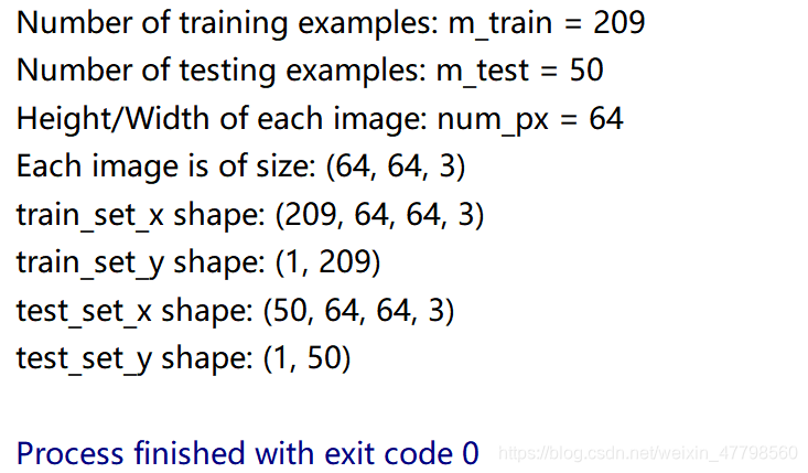
print ("Number of training examples: m_train = " + str(m_train))
print ("Number of testing examples: m_test = " + str(m_test))
print ("Height/Width of each image: num_px = " + str(num_px))
print ("Each image is of size: (" + str(num_px) + ", " + str(num_px) + ", 3)")
print ("train_set_x shape: " + str(train_set_x_orig.shape))
print ("train_set_y shape: " + str(train_set_y_orig.shape))
print ("test_set_x shape: " + str(test_set_x_orig.shape))
print ("test_set_y shape: " + str(test_set_y_orig.shape))

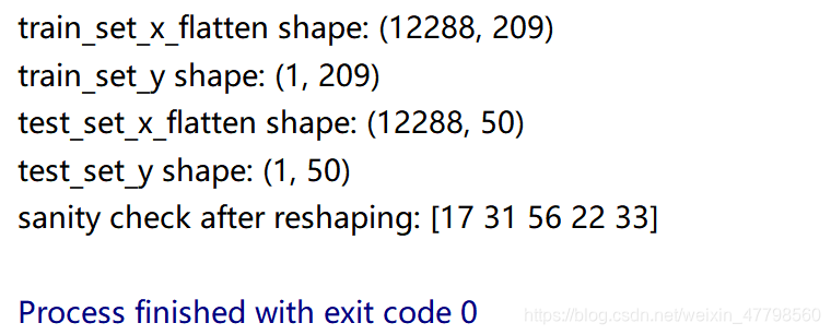
练习： 重塑训练和测试数据集，以便将大小（num_px，num_px，3）的图像展平为单个形状的向量(num_px * num_px * 3, 1)。

train_set_x_flatten = train_set_x_orig.reshape(train_set_x_orig.shape[0], -1).T
test_set_x_flatten = test_set_x_orig.reshape(test_set_x_orig.shape[0], -1).T

print ("train_set_x_flatten shape: " + str(train_set_x_flatten.shape))
print ("train_set_y shape: " + str(train_set_y_orig.shape))
print ("test_set_x_flatten shape: " + str(test_set_x_flatten.shape))
print ("test_set_y shape: " + str(test_set_y_orig.shape))
print ("sanity check after reshaping: " + str(train_set_x_flatten[0:5,0]))

为了表示彩色图像，必须为每个像素指定红、绿、蓝色通道（RGB），因此像素值实际上是一个从0到255的三个数字的向量。

机器学习中一个常见的预处理步骤是对数据集进行居中和标准化，这意味着你要从每个示例中减去整个numpy数组的均值，然后除以整个numpy数组的标准差。但是图片数据集则更为简单方便，并且只要将数据集的每一行除以255（像素通道的最大值），效果也差不多。

在训练模型期间，你将要乘以权重并向一些初始输入添加偏差以观察神经元的激活。然后，使用反向梯度传播以训练模型。但是，让特征具有相似的范围以至渐变不会爆炸是非常重要的。具体内容我们将在后面的教程中详细学习！

train_set_x = train_set_x_flatten / 255
test_set_x = test_set_x_flatten / 255
train_set_y = train_set_y_orig
test_set_y = test_set_y_orig

你需要记住的内容：

预处理数据集的常见步骤是：

1. 找出数据的尺寸和维度（m_train，m_test，num_px等）
2. 重塑数据集，以使每个示例都是大小为（num_px \ num_px \ 3，1）的向量
3. “标准化”数据

3 学习算法的一般架构

现在是时候设计一种简单的算法来区分猫图像和非猫图像了。

你将使用神经网络思维方式建立Logistic回归。 下图说明了为什么“逻辑回归实际上是一个非常简单的神经网络！”

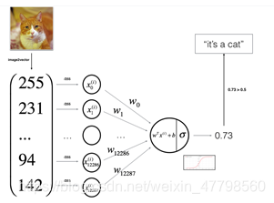
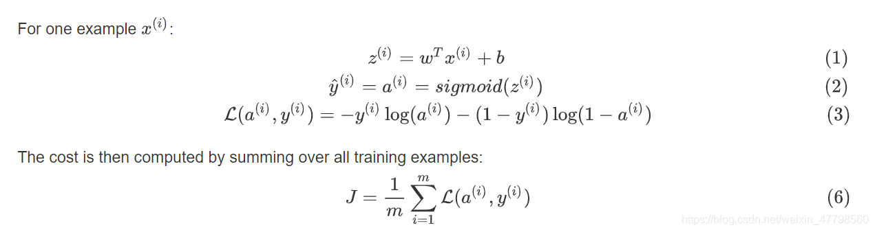
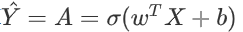
算法的数学表达式：

关键步骤：
在本练习中，你将执行以下步骤：

 初始化模型参数
 通过最小化损失来学习模型的参数
 使用学习到的参数进行预测（在测试集上）
 分析结果并得出结论

4 构建算法的各个部分

建立神经网络的主要步骤是：
1.定义模型结构（例如输入特征的数量）
2.初始化模型的参数
3.循环：

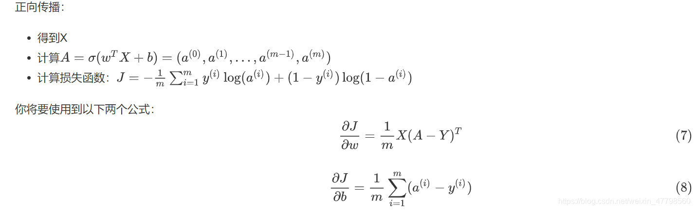
 计算当前损失（正向传播）
 计算当前梯度（向后传播）
 更新参数（梯度下降）

你通常会分别构建1-3，然后将它们集成到一个称为“ model（）”的函数中。

4.1 辅助函数

练习：使用“Python基础”中的代码，实现sigmoid（）。 如上图所示，你需要计算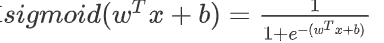
去预测。 使用np.exp（）。

def sigmoid(z):
    s = 1 / (1 + np.exp(-z))
    return s

4.2 初始化参数

练习： 在下面的单元格中实现参数初始化。 你必须将w初始化为零的向量。 如果你不知道要使用什么numpy函数，请在Numpy库的文档中查找np.zeros（）。

def initializee_with_zeros(dim):
    w = np.zeros((dim,1))
    b = 0
    return w,b
    
dim = 2
w, b = initialize_with_zeros(dim)
print ("w = " + str(w))
print ("b = " + str(b))

4.3 前向和后向传播

练习： 实现函数propagate（）来计算损失函数及其梯度。
提示：

def propagate(w,b,x,y):
"""
    Implement the cost function and its gradient for the propagation explained above

    Arguments:
    w -- weights, a numpy array of size (num_px * num_px * 3, 1)
    b -- bias, a scalar
    X -- data of size (num_px * num_px * 3, number of examples)
    Y -- true "label" vector (containing 0 if non-cat, 1 if cat) of size (1, number of examples)

    Return:
    cost -- negative log-likelihood cost for logistic regression
    dw -- gradient of the loss with respect to w, thus same shape as w
    db -- gradient of the loss with respect to b, thus same shape as b
    
    Tips:
    - Write your code step by step for the propagation. np.log(), np.dot()
    """
    m = x.shape[1]
    a = sigmoid(w.T @ x + b)
    cost = - 1 / m * np.sum(y * np.log(a) +(1-y) * np.log(1-a))
    dw = 1 / m * x @ (a - y).T
    db = 1 / m * np.sum(a - y)
    return cost,dw,db

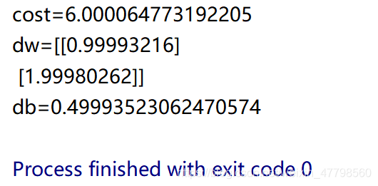
w, b, x, y = np.array([[1],[2]]), 2, np.array([[1,2],[3,4]]), np.array([[1,0]])
cost,dw,db = propagate(w,b,x,y)
print('cost='+str(cost))
print('dw='+str(dw))
print('db='+str(db))

优化函数

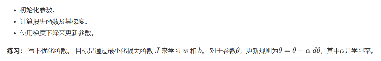
def optimize(w,b,x,y,iterations,learning_rate):

    for i in range(iterations):
        cost,dw,db = propagate(w,b,x,y)
        w = w - learning_rate * dw
        b = b - learning_rate * db

    return w,b,dw,db

w,b,dw,db = optimize(w,b,x,y,100,0.02)
print(w,b,dw,db)

练习： 上一个函数将输出学习到的w和b。 我们能够使用w和b来预测数据集X的标签。实现**predict（）**函数。 预测分类有两个步骤：
1.计算

2.将a的项转换为0（如果激活<= 0.5）或1（如果激活> 0.5），并将预测结果存储在向量“ Y_prediction”中。 如果愿意，可以在for循环中使用if / else语句。

def predict(w,b,x,y):
    m = x.shape[1]
    y_predict = np.zeros((1,m))
    w = w.reshape(x.shape[0],1)
    a = sigmoid(w.T @ x + b)
    for i in range(a.shape[1]):
        if a[0,i] > 0.5:
            y_predict[i] = 1
    return y_predict

print(predict(w,b,x,y))

你需要记住以下几点：
你已经实现了以下几个函数：

初始化（w，b）
迭代优化损失以学习参数（w，b）：
计算损失及其梯度
使用梯度下降更新参数
使用学到的（w，b）来预测给定示例集的标签

5 将所有功能合并到模型中

练习： 实现模型功能，使用以下符号：

 Y_prediction对测试集的预测
 Y_prediction_train对训练集的预测
 w，损失，optimize（）输出的梯度

def model(train_set_x,train_set_y,test_set_x,test_set_y):
    w,b = initializee_with_zeros(train_set_x.shape[0])
    cost,dw,db = propagate(w,b,train_set_x,train_set_y)
    w, b, dw, db = optimize(w, b, train_set_x, train_set_y, 100, 0.02)
    y_train = predict(w,b,train_set_x)
    y_train_acc =np.mean(np.abs(y_train - train_set_y)) * 100
    y_test = predict(w,b,test_set_x)
    y_test_acc = np.mean(np.abs(y_test - test_set_y)) * 100
    return y_train,y_train_acc,y_test,y_test_acc

print(model(train_set_x,train_set_y,test_set_x,test_set_y))