


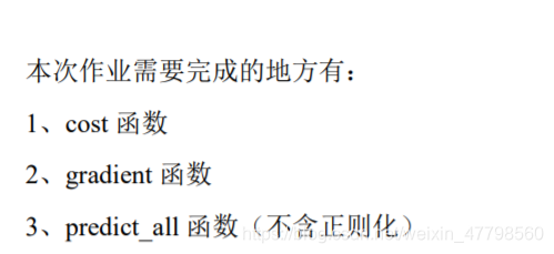
吴恩达机器学习作业三:多类分类
知识点回顾:
import numpy as np
import pandas as pd
import matplotlib.pyplot as plt
from scipy.io import loadmat
1.1 Dataset
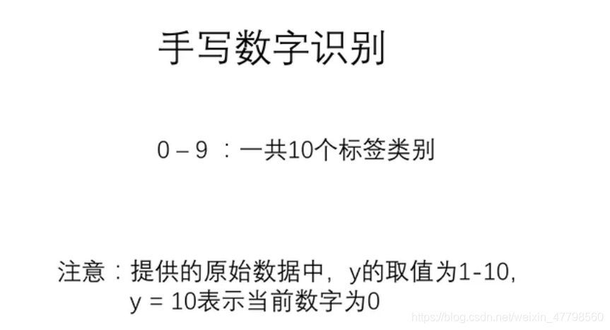
原始数据集的标签 y, y取值为1到10,y = 10表示当前手写字为0,其余1到9即对应1到9。
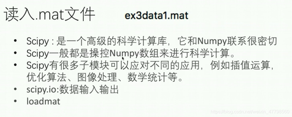
数据集保存在 ex3data1.mat,注意文件格式跟之前不一样,用matlab打开可以看到有X和y两个变量:
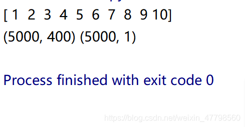
X的维度是5000×400,表示有5000个样本,每个样本有400个特征(其实就是20×20的像素值);
y的维度是5000×1,表示有5000个样本,每个样本对应1个标签(1到10共十种标签值,每种标签有500个样本)
首先,加载数据集。这里的数据为MATLAB的格式,所以要使用SciPy.io的loadmat函数。作业中为了导入数据,代码使用了 scipy.io 库。这是一个可以帮助我们导入.mat 格式数据的包。
def load_data(path):
    data = loadmat(path)
    x = data['X']
    y = data['y']
    return x,y
path = 'D:\编程\ex3data1.mat'
x,y = load_data(path)
# 看看有几类标签
print(np.unique(y))
print(x.shape,y.shape)
"""
每个训练样本是一个20x20的图像
原始数据是一个字典,字典中的X的shape是(5000,400),y的shape是(5000,1)
X的每一行代表一个数字图像的特征向量(400维,一个像素占一维)
y(1,2,3···9,10)代表数字的值(1,2,3···9,0),共有5000个训练样本
"""
1.2 Visualizing the data
矩阵显示:matshow()函数
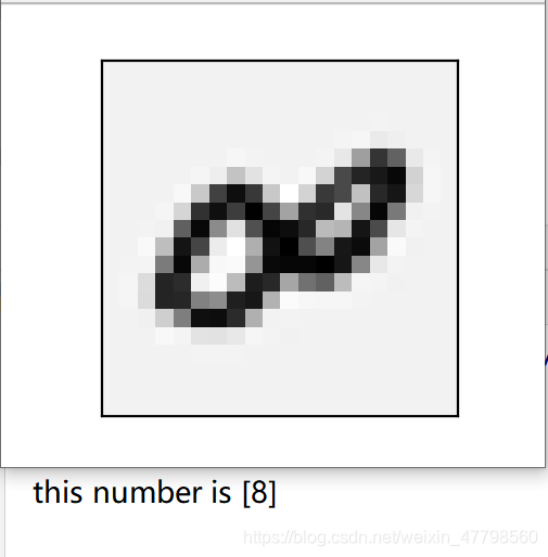
pick_one =np.random.randint(0,5000)
print('this number is {}'.format(y[pick_one]))
image = x[pick_one,:]
'''
fig, ax = plt.subplots()等价于:
fig = plt.figure()
ax = fig.add_subplot(1, 1, 1)

'''
fig, ax = plt.subplots(figsize=(3, 3))
ax.matshow(image.reshape((20, 20)), cmap='gray_r')
# 去除刻度,美观,函数plt.xticks()和plt.xticks()用来实现对x轴和y轴坐标间隔(也就是轴记号)的设定
plt.xticks([])
plt.yticks([])
plt.show()
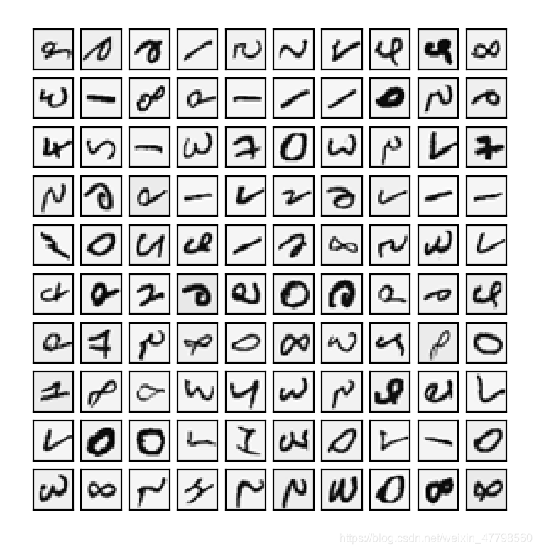
def plot_100_image(X):
    """
    随机画100个数字
    """
    sample_idx = np.random.choice(np.arange(X.shape[0]), 100)  # 随机选100个样本
    sample_images = X[sample_idx, :]  # (100,400)
    fig, ax_array = plt.subplots(nrows=10, ncols=10, sharey=True, sharex=True, figsize=(8, 8))
    for row in range(10):
        for column in range(10):
            ax_array[row, column].matshow(sample_images[10 * row + column].reshape((20, 20)),
                                          cmap='gray_r')
    plt.xticks([])
    plt.yticks([])
    plt.show()

print(plot_100_image(x))
1.3 Vectorizing Logistic Regression
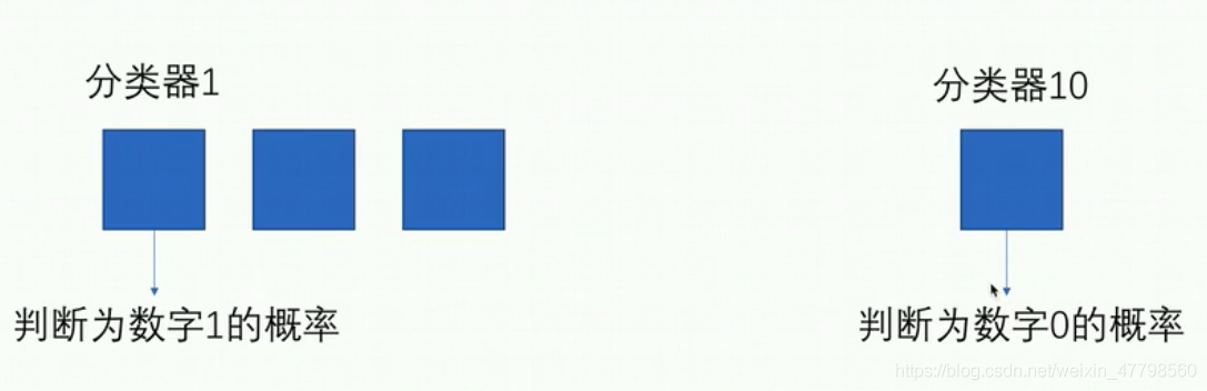
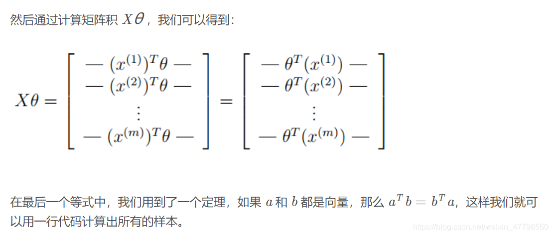
我们将使用多个one-vs-all(一对多)logistic回归模型来构建一个多类分类器。由于有10个类,需要训练10个独立的分类器。为了提高训练效率,重要的是向量化。在本节中,我们将实现一个不使用任何for循环的向量化的logistic回归版本。
首先准备下数据。
准备数据
x = np.insert(x, 0, values=1, axis=1)  # 在首列插入x0=1的一列。axis=1表示按列插入
y = y.flatten()  # 使得到的 y为一维数组
print(x.shape)
print(y.shape)
1.3.1 Vectorizing the cost function
# 向量化代价函数
# 定义logistic函数
def sigmoid(z):
    return 1/(1+np.exp(-z))

def regular_costf(x,y,theta,lam):
    first = - y * np.log(sigmoid(x @ theta))
    second = -(1-y) * np.log(1-sigmoid(x @ theta))
    third = theta[1:]
    return np.mean(first+second)+ np.sum(np.power(third,2)) *(lam/(2*len(x)))
1.3.2 Vectorizing the gradient
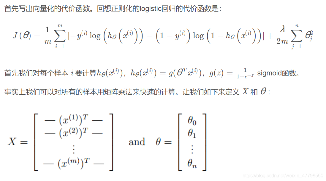
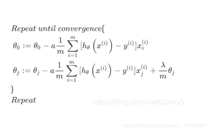
回顾正则化logistic回归代价函数的梯度下降法如下表示,因为不惩罚theta_0,所以分为两种情况:
# 梯度下降算法
def regular_gradient(x,y,theta,lam):
    gradient =(x.T @ (sigmoid(x @ theta) - y))/len(x)
    reg = theta * (lam/len(x))
    reg[0] = 0
    return gradient+reg
1.4 One-vs-all Classification
这部分我们将实现一对多分类通过训练多个正则化logistic回归分类器,每个对应数据集中K类中的一个。
对于这个任务,我们有10个可能的类,并且由于logistic回归只能一次在2个类之间进行分类,每个分类器在“类别 i”和“不是 i”之间决定。 我们将把分类器训练包含在一个函数中,该函数计算10个分类器中的每个分类器的最终权重,并将权重返回shape为(k, (n+1))数组,其中 n 是参数数量。
from scipy.optimize import minimize


def one_vs_all(X, y, l, K):
    """generalized logistic regression
    args:
        X: feature matrix, (m, n+1) # with incercept x0=1
        y: target vector, (m, )
        l: lambda constant for regularization
        K: numbel of labels
    return: trained parameters
    """
    all_theta = np.zeros((K, X.shape[1]))  # (10, 401)

    for i in range(1, K + 1):
        theta = np.zeros(X.shape[1])
        y_i = np.array([1 if label == i else 0 for label in y])

        ret = minimize(fun=regular_costf, x0=theta, args=(X, y_i, l), method='TNC',
                       jac=regular_gradient, options={'disp': True})
        all_theta[i - 1, :] = ret.x

    return all_theta
l =1
k =10
all_theta = one_vs_all(x,y,l,k)
这里需要注意的几点:首先,我们为theta添加了一个额外的参数(与训练数据一列),以计算截距项(常数项)。 其次,我们将y从类标签转换为每个分类器的二进制值(要么是类i,要么不是类i)。 最后,我们使用SciPy的较新优化API来最小化每个分类器的代价函数。 如果指定的话,API将采用目标函数,初始参数集,优化方法和jacobian(渐变)函数。 然后将优化程序找到的参数分配给参数数组。
实现向量化代码的一个更具挑战性的部分是正确地写入所有的矩阵,保证维度正确。
注意,theta是一维数组,因此当它被转换为计算梯度的代码中的矩阵时,它变为(1×401)矩阵。 我们还检查y中的类标签,以确保它们看起来像我们想象的一致。
我们现在准备好最后一步 - 使用训练完毕的分类器预测每个图像的标签。 对于这一步,我们将计算每个类的类概率,对于每个训练样本(使用当然的向量化代码),并将输出类标签为具有最高概率的类。
Tip:可以使用np.argmax()函数找到矩阵中指定维度的最大值
def predict(x, all_theta):
    # 5000个样本,每个样本都有10个预测输出(概率值)
    h = sigmoid(x @ all_theta.T)  # (5000,401) (10,401)^T=>(5000,10)

    # 每个样本取自己10个预测中最大的值作为最终预测值
    h_argmax = np.argmax(h, axis=1)  # 按列比较,argmax表示返回该行最大值对应的列索引

    return h_argmax + 1  # 返回列索引为0表示标签值为1,返回列索引为9表示标签值为10(代表数字0)


y_pre = predict(x, all_theta)
acc = np.mean(y_pre == y)
print('accuracy = {0}%'.format(acc * 100))
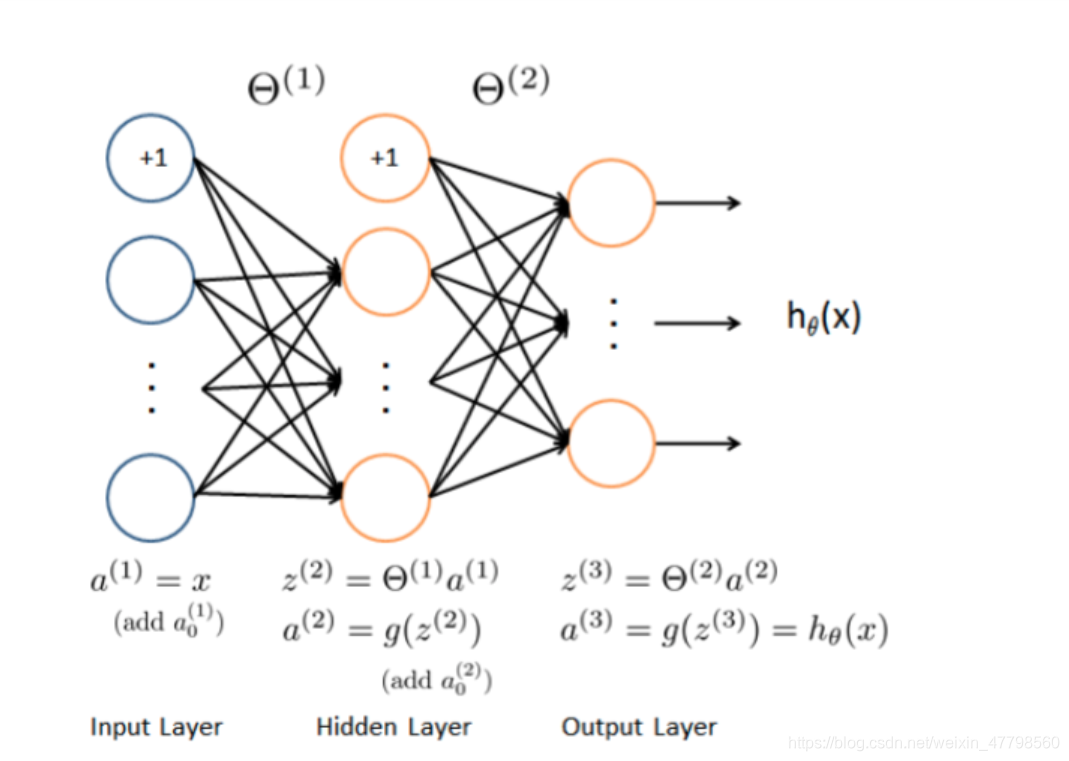
2 Neural Networks
上面使用了多类logistic回归,然而logistic回归不能形成更复杂的假设,因为它只是一个线性分类器。
接下来我们用神经网络来尝试下,神经网络可以实现非常复杂的非线性的模型。我们将利用已经训练好了的权重进行预测。
案例: 手写数字识别
数据集:ex3data1.mat
参数集:ex3weights.mat
题目和数据集不变,但直接给出了神经网络的训练参数结果,所以本练习只是简单用代码了解神经网络的前向传播过程,不涉及训练过程。
2.1 获取数据集
import numpy as np
from scipy.io import loadmat

def load_data(path):
    data = loadmat(path)
    x = data['X']
    y = data['y']
    return x,y
path = 'D:\编程\ex3data1.mat'
x = np.insert(x,0,values = 1,axis =1)  #(5000,401)
y = y.flatten()  #(5000,)
2.2 获取训练参数
path_theta = 'D:\编程\ex3weights.mat'
theta = loadmat(path_theta)
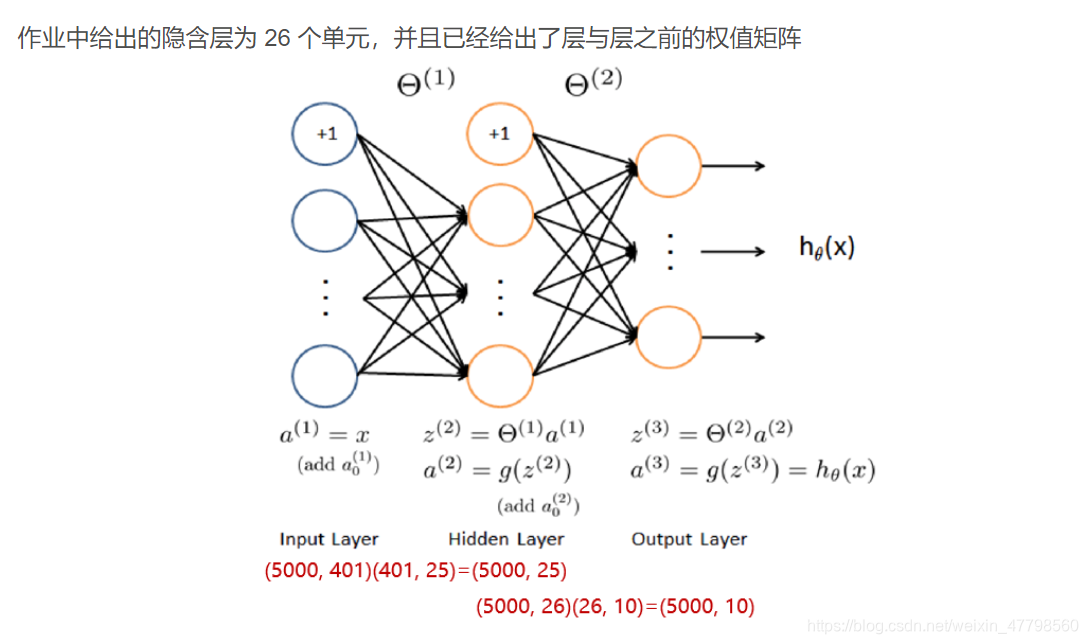
theta1 = theta['Theta1'] # (25, 401)
theta2 = theta['Theta2'] # (10, 26)
print(theta1.shape)
print(theta2.shape)
2.3 前向传播过程
# 定义激活函数
def sigmoid(z):
    return 1 / (1 + np.exp(-z))

# 输入层
a1 = x # a1.shape=(5000, 401)

# 隐藏层
z2 = x @ theta1.T  # (5000, 401)(401, 25) = (5000, 25)
a2 = sigmoid(z2)  # a2.shape=(5000, 25)

# 输出层
a2 = np.insert(a2, 0, values=1, axis=1)  # (5000, 26)
z3 = a2 @ theta2.T  # (5000, 26)(26, 10) = (5000, 10)
a3 = sigmoid(z3)  # a3.shape=(5000, 10)
2.4 计算分类准确率
上一步得到的a3维度是(5000, 10),即5000个样本,每个样本都输出10个预测输出(概率值)
# 同1.3节
y_pre = np.argmax(a3,axis=1)
y_pre = y_pre + 1
# 计算分类准确率
acc = np.mean(y_pre == y)
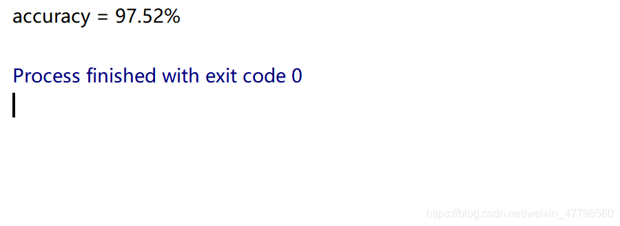
print('accuracy = {}%'.format(acc * 100))


 709
709

 被折叠的 条评论
为什么被折叠?
被折叠的 条评论
为什么被折叠?
 到【灌水乐园】发言


