手写支持向量机(SVM)实例之——鸢尾花卉数据集分割

鸢尾花（iris）是单子叶百合目花卉，是一种比较常见的花，可能不经意间你就能在某个公园里碰见它，而且鸢尾花的品种较多。该数据集是机器学习领域相当经典的一个小数据集，仅有150行，5列。该数据集的四个特征属性的取值都是数值型的，他们具有相同的量纲，不需要你做任何标准化的处理，第五列为通过前面四列所确定的鸢尾花所属的类别名称。

1. 数据集展示及问题描述

iris数据集本身集成在sklearn包中，在安装这个包的时候，本身就会安装这个数据集。我们首先来简单看一下这个数据集。

from sklearn.datasets import load_iris
data = load_iris()	#获得数据本身
print(data.keys())	#数据集中包含什么
#dict_keys(['data', 'target', 'frame', 'target_names', 'DESCR', 'feature_names', 'filename', 'data_module'])

print(data.target_names)
#['setosa' 'versicolor' 'virginica']

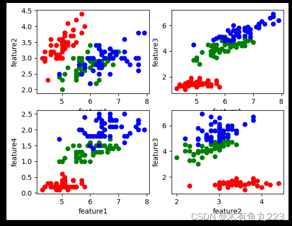
这个数据集本身很简单，共150条数据，分为三类(setosa、versicolor、virginica)，每条数据特征有4条(四个长度)。简单来说，这个数据集就是根据一朵花，测量出来的四个长度，然后判断它属于三类中的哪一类。画个图解释一下。

data = iris['data']
target = iris['target']

sp1 = data[target == 0]
sp2 = data[target == 1]
sp3 = data[target == 2]
plt.subplot(221)
plt.scatter(x = sp1[:, 0], y = sp1[:, 1], color = "red")
plt.scatter(x = sp2[:, 0], y = sp2[:, 1], color = "green")
plt.scatter(x = sp3[:, 0], y = sp3[:, 1], color = "blue")
plt.xlabel("feature1")
plt.ylabel("feature2")

plt.subplot(222)
plt.scatter(x = sp1[:, 0], y = sp1[:, 2], color = "red")
plt.scatter(x = sp2[:, 0], y = sp2[:, 2], color = "green")
plt.scatter(x = sp3[:, 0], y = sp3[:, 2], color = "blue")
plt.xlabel("feature1")
plt.ylabel("feature3")
plt.subplot(223)
plt.scatter(x = sp1[:, 0], y = sp1[:, 3], color = "red")
plt.scatter(x = sp2[:, 0], y = sp2[:, 3], color = "green")
plt.scatter(x = sp3[:, 0], y = sp3[:, 3], color = "blue")
plt.xlabel("feature1")
plt.ylabel("feature4")
plt.subplot(224)
plt.scatter(x = sp1[:, 1], y = sp1[:, 2], color = "red")
plt.scatter(x = sp2[:, 1], y = sp2[:, 2], color = "green")
plt.scatter(x = sp3[:, 1], y = sp3[:, 2], color = "blue")
plt.xlabel("feature2")
plt.ylabel("feature3")
plt.show()

2. SVM模型构建及训练

这里调用一下sklearn库中的SVC，嗯，真香。不是我不写，主要是因为SMO算法我还没看懂。

from sklearn.model_selection import train_test_split
from sklearn.svm import SVC
from sklearn.model_selection import train_test_split

x_train, x_test, y_train, y_test = train_test_split(data, target, test_size = 0.2, random_state = 42)
ssvc = SVC(kernel = 'linear', C = 1).fit(x_train, y_train)
print(ssvc.score(data, target))
print(ssvc.score(x_train, y_train))
print(ssvc.score(x_test, y_test))

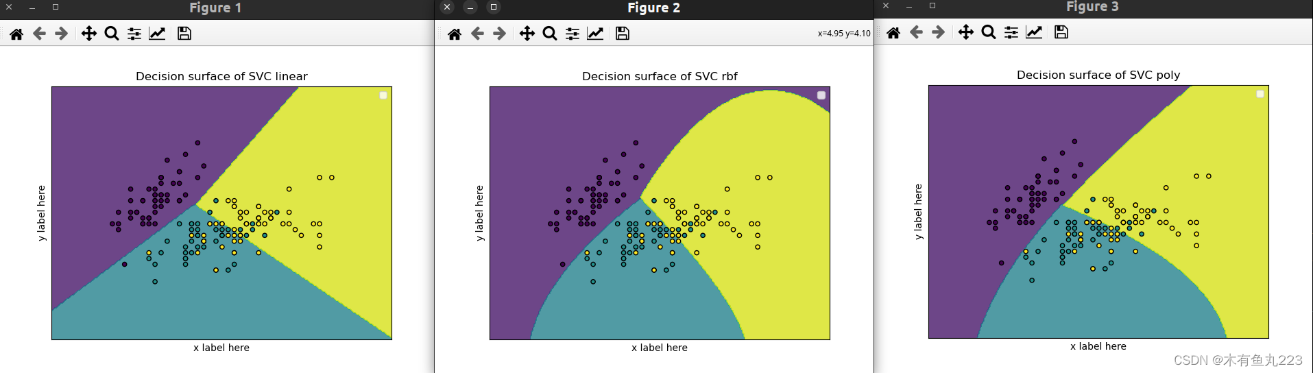
3. 使用不同的核函数

本部分使用了线性核函数，多项式核函数以及高斯核函数，分别进行训练。

from sklearn.svm import SVC
from sklearn.metrics import accuracy_score
import matplotlib.pyplot as plt
import numpy as np
from sklearn.model_selection import train_test_split
from sklearn.datasets import load_iris

# Input the kernel from the user

def make_meshgrid(x, y, h=.02):
    x_min, x_max = x.min() - 1, x.max() + 1
    y_min, y_max = y.min() - 1, y.max() + 1
    xx, yy = np.meshgrid(np.arange(x_min, x_max, h), np.arange(y_min, y_max, h))
    return xx, yy

def plot_contours(ax, clf, xx, yy, **params):
    Z = clf.predict(np.c_[xx.ravel(), yy.ravel()])
    Z = Z.reshape(xx.shape)
    out = ax.contourf(xx, yy, Z, **params)
    return out


if __name__ == '__main__':
    iris = load_iris()
    x = iris.data[:, 0:2]
    y = iris.target
    X_train, X_test, y_train, y_test = train_test_split(x, y, test_size=0.55, random_state=42)
    kernels = ['linear', 'rbf', 'poly']
    for  kernel in kernels:
        model = SVC(kernel= kernel)
        model.fit(X_train, y_train)

        pred = model.predict(X_test)

        print("Accuracy using {}:".format(kernel), accuracy_score(pred, y_test))
        
        fig, ax = plt.subplots()
        # title for the plots
        title = ('Decision surface of SVC ' + model.kernel)
        # Set-up grid for plotting.
        X0, X1 = x[:, 0], x[:, 1]
        xx, yy = make_meshgrid(X0, X1)

        plot_contours(ax, model, xx, yy, alpha=0.8)
        ax.scatter(X0, X1, c=y, s=20, edgecolors='k')
        ax.set_ylabel('y label here')
        ax.set_xlabel('x label here')
        ax.set_xticks(())
        ax.set_yticks(())
        ax.set_title(title)
        ax.legend()
    plt.show()