【全局敏感性分析】【基于密度的灵敏度指数】【不确定性分析】基于累积分布函数的全局敏感性分析的简单高效方法（Matlab代码实现）

💥1 概述

摘要

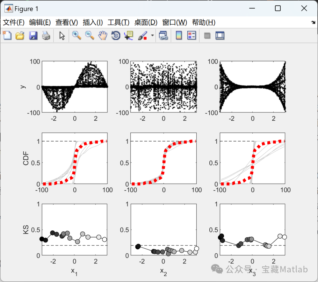
基于方差的方法被广泛用于环境模型的全局敏感性分析（GSA）。然而，在输出分布高度倾斜或具有多峰性的情况下，考虑模型输出的整个概率密度函数（PDF），而不仅是其方差的方法，更为合适，因为方差可能无法充分代表不确定性。尽管如此，基于密度的方法的采用至今仍相对有限，可能因为其相对更难实现。在本文中，我们介绍一种名为PAWN的新型GSA方法，用于高效计算基于密度的灵敏度指数。其关键思想是通过累积分布函数（CDF）表征输出分布，相对于PDF来说，CDF更易于推导。我们讨论并演示了PAWN的优势，通过数值和环境建模示例的应用。我们期望PAWN能够促进基于密度的方法的应用，并作为基于方差的GSA的补充方法。

关键词 全局敏感性分析、基于方差的灵敏度指数、基于密度的灵敏度指数、不确定性分析

全局敏感性分析（GSA）是一组数学技术，旨在评估不确定性通过数值模型的传播，特别是理解不同不确定性来源对模型输出变异性的相对贡献。定量GSA使用灵敏度指数，将这样的相对影响总结为一个标量度量。不确定性来源可能包括模型参数、外部数据误差，甚至非数值不确定性，如空间分布模拟模型格网的分辨率。

一种成熟且广泛应用的GSA方法是基于方差的方法。在这里，对不确定输入的输出灵敏度是通过来自该输入不确定性的输出方差贡献来衡量的。基于方差的灵敏度指数在不同环境建模领域的GSA应用中越来越受欢迎（例如，参见Pastres等人，1999年; Pappenberger等人，2008年; van Werkhoven等人，2008年; Nossent等人，2011年; Ziliani等人，2013年; Baroni和Tarantola，2014年，以及Saltelli等人（2008年）以获取更多一般性讨论）。它们传播的主要原因在于拥有几个可取的属性，特别是：它们可独立于输入-输出响应函数的特性（例如线性或非线性）应用; 它们可用于输入排序（即所谓的“因子优先级”）和筛选; 它们易于实施和解释。

详细文章见第4部分。

📚2 运行结果

部分代码：

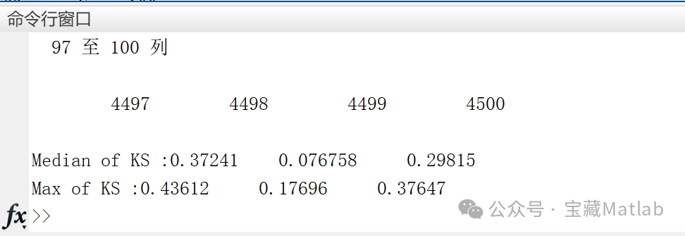
function [KS,xvals,y_u, y_c, par_u, par_c, ft] = PAWN(model, p, lb, ub, ...Nu, n, Nc, npts, seed)%PAWN Run PAWN for Global Sensitivity Analysis of a supplied model%   [KS,xvals,y_u, y_c, par_u, par_c, ft] = PAWN(model, p, lb, ub, ...% Nu, n, Nc, npts, seed)%%     model : A function that takes a vector of parameters x and a %             structure p as input to provide the model output as a scalar.%             The vector holds parameters we need sensitivity of and p%             holds all other parameters required to run the model.%     lb : A vector (1xM) of the lower bounds for each parameter%     ub : A vector (1xM) of the upper bounds for each parameter%     Nu : Number of samples of the unconditioned parameter space%     n : Number of conditioning values in each dimension%     Nc : Number of samples of the conditioned parameter space%     npts : Number of points to use in kernel density estimation%     seed : Random number seed    % Initializations    M = length(lb); % Number of parameters    y_u = nan(Nu,1); % Ouput of unconditioned simulations    y_c = n * Nc * M; % Output of conditioned simulations    KS = nan(M,n); % Kolmogorov-Smirnov statistic    xvals = nan(M,n); % Container for conditioned samples    ft = nan(M*n, npts); % CDF container    rng(seed); % Set random seed    % Containers for parameters    par_u = bsxfun(@plus, lb, bsxfun(@times, rand(Nu, M), (ub-lb)));                     par_c = bsxfun(@plus, lb, bsxfun(@times, rand(M*Nc*n, length(lb)), (ub-lb)));    % Create the conditioned samples    for ind=1:M        for ind2=1:n            xvals(ind,ind2) = lb(ind) + rand*(ub(ind)-lb(ind));            [(ind-1)*Nc*n+(ind2-1)*Nc+1:(ind-1)*Nc*n+ind2*Nc]            par_c((ind-1)*Nc*n+(ind2-1)*Nc+1:...                (ind-1)*Nc*n+ind2*Nc,ind) = xvals(ind,ind2);        end    end    % Evaluate model output of unconditioned samples, can parallelize by    % commenting out the parfor line and adding a comment to the for line.%     parfor ind=1:Nu    for ind=1:Nu        y_u(ind) = model(par_u(ind,:), p);    end    % Evaluate model output of conditioned samples, can parallelize by    % commenting out the parfor line and adding a comment to the for line.%     parfor ind=1:length(par_c)    for ind=1:length(par_c)        y_c(ind) = model(par_c(ind,:), p);    end    % Find bounds of the model outputs    m1 = min([y_c, y_u']);    m2 = max([y_c, y_u']);    % Evaluate the CDF with kernel density for unconditioned samples    [f,~] = ksdensity(y_u, linspace(m1,m2,npts), 'Function', 'cdf');    % Evaluate the CDF with kernel density for conditioned samples and use    % that to find the KS statistic (Eqn 4 in the paper).     for ind=1:M        for ind2=1:n            % Temporarily store the current conditioned samples            yt = y_c((ind-1)*Nc*n+(ind2-1)*Nc+1:(ind-1)*Nc*n+ind2*Nc);            [ft((ind-1)*n+ind2,:),~] = ksdensity(yt, linspace(m1, m2,...                                                 npts), 'Function', 'cdf');            KS(ind,ind2) = max(abs(ft((ind-1)*n+ind2,:)-f)); % Eqn 4        end    endend

🎉3 参考文献

文章中一些内容引自网络，会注明出处或引用为参考文献，难免有未尽之处，如有不妥，请随时联系删除。

[1]: Pianosi, F., Wagener, T., 2015. A simple and efficient method for 

global sensitivity analysis based on cumulative distribution functions. 

Environ. Model. Softw. 67, 1-11. doi:10.1016/j.envsoft.2015.01.004

🌈4 Matlab代码、文献