基于神经网络的QMF滤波器设计

基于神经网络的2通道正交镜像滤波器组设计

1 | 引言

双通道正交镜像滤波（QMF）滤波器组因其高效的多相实现以及灵活的频率特性而受到广泛关注和研究。在过去几十年中，正交镜像滤波器组已广泛应用于各种信号处理领域1-7，包括音频和语音的子带编码、通信系统、图像压缩、小波基设计、生物医学工程以及多速率信号处理系统。在设计双通道QMF滤波器组时，必须消除或最小化三种类型的失真：混叠失真、幅度失真和相位失真。传统上，通过有限冲激响应或无限冲激响应（IIR）滤波器适当设计构成QMF滤波器组系统基础的低通分析原型滤波器，以消除混叠失真。直接优化原型滤波器会带来高度非线性的非线性优化问题7，因此无法保证分析滤波器系数的最优设计。此外，原型滤波器的设计会同时产生幅度和相位失真。

最近的研究7-29表明，无混叠的双通道QMF滤波器组可以通过一系列互连的IIR全通滤波器有效构建。由于 IIR全通滤波器能够保持单位幅度和规定相位，因此QMF滤波器组设计可简化为求解全通滤波器的相位逼近问题，而不会产生幅度失真。因此，基于IIR全通滤波器的QMF滤波器组设计具有较低的计算负担，且所设计的性能在多个方面优于有限冲激响应原型滤波器设计。13

劳森和克鲁切‐杰迪德11,12提出了一种计算高效的优化方法，分别优化正切相位函数的分子和分母，从而得到一个闭式表达式。由于所设计的两个IIR全通滤波器具有符号相反的相同系数，滤波器的灵活性和设计精度受到较大限制，因此整体QMF滤波器组导致较大的相位误差和群延迟响应。在文献中，15 QMF滤波器组设计问题被表述为基于非线性极小极大算法并结合卡马尔卡尔算法的一种变体来求解IIR全通滤波器的实值系数。通过频率采样和迭代逼近方法可高效地获得最优滤波器系数。然而，本文提出的算法在最小化过程中需要反复进行矩阵求逆，因此随着滤波器长度的增加，计算复杂度显著上升。

在先前的研究中，25作者提出了一种基于神经小成分分析的替代算法，用于设计具有精确性能和简单性的IIR 全通型QMF滤波器组。该神经学习规则通过迭代实现对应于设计规范协方差矩阵最小特征值的特征滤波器设计。由于仅需计算一个特征向量，该设计流程是高效的。然而，设计性能主要受限于合适参考频率的选择。在文献中，26全通型QMF滤波器组通过求解与Toeplitz加Hankel矩阵相关的线性方程组的闭式解来实现。基于线性代数的简化结合三角恒等式可显著降低计算负担并实现精确性能。

最小二乘法（LS）9,26,30-38和极小极大逼近36,39在IIR全通滤波器的设计中被广泛研究。由于目标函数的高度非线性，上述数值方法可能无法实现最优设计。因此，已提出若干方法，如非线性、受自然启发的以及无需导数的优化技术35,37,38,40-48，用于设计各类性能更优的数字滤波器。在文献中，35,37,44,46作者应用反馈神经网络49-52显著降低了计算负担，并精确获得了与其他方法相同的设计结果。40,42基于神经网络的方法的优点包括快速收敛、优异的数值逼近能力以及实时处理能力。尽管受自然启发的优化技术也具备这些优点，但其主要问题在于原型滤波器的非线性优化求解，因此计算效率受到完全限制。

在数字信号处理领域中，设计具有低重建误差和低群延迟的双通道QMF滤波器组起着至关重要的作用，并受到越来越多的关注和应用。本文利用一种规则且简化的霍普菲尔德神经网络结构，实现了基于IIR全通滤波器的 QMF滤波器组的最小二乘设计，具有较高的精度和有效性。本文结构如下：第二节简要介绍了基于IIR全通滤波器的双通道QMF滤波器组的最小二乘设计；第三节详细阐述了应用于基于实值IIR全通滤波器的双通道QMF滤波器组设计的霍普菲尔德神经网络；第四节将仿真结果与传统最小二乘方法设计的结果进行比较，以展示本文提出的神经网络算法的性能；最后，第五节给出本文的结论。

使用全通滤波器的QMF滤波器组设计问题的表述

双通道QMF滤波器组的系统架构由分析系统和综合系统组成，如图1所示。在分析系统中，信号分别通过低通滤波器H0(z)和高通滤波器H1(z)被分解为1个低频分量和1个高频分量。双通道QMF滤波器组的重建信号可简单表示为

$$
\hat{X}(z) = \frac{1}{2} [H_0(z)G_0(z) + H_1(z)G_1(z)]X(z) + \frac{1}{2} [H_0(-z)G_0(z) + H_1(-z)G_1(z)]X(-z); \tag{1}
$$

其中第一项表示期望的线性时不变响应，第二项表示由于采样率转换引起的混叠失真。

由于H1(z)相对于四分之一频率 ω= π/2是H0(z)的镜像，因此满足关系式H0(z) = H1(−z)。在综合系统中，通过适当地选择综合滤波器以满足G0(z) = H1(−z)和G1(z) = −H0(−z)的条件，可以完全消除混叠失真。因此，无混叠的双通道QMF滤波器组的传输函数可表示为15,25,26,46

$$
\hat{X}(z) = \frac{1}{2} H_0^2(-z) X(z) = \frac{1}{2}M(z) X(z): \tag{2}
$$

显然，双通道QMF滤波器组可以通过设计单一的低通分析滤波器H0(z)进行等效简化。此外，重建信号的幅值质量也很大程度上依赖于低通滤波器H0(z)的设计。因此，M(ejω)必须具有线性相位响应并满足纯延迟，以减小幅度失真。然而，在最小二乘意义下将M(ejω)逼近为单位幅值响应时，会得到一个关于低通分析滤波器的四次函数。这涉及高度非线性优化，并且计算成本显著增加，因此难以保证获得最优设计。

在一些研究中，9,12,15,17-20,23,25,26 IIR全通滤波器的互连结构在双通道QMF滤波器组的完全重建设计中引起了广泛关注。利用IIR全通滤波器设计QMF滤波器组具有诸多优点，包括近似线性相位响应、较低的计算负担、高效的多相实现方式，并且不会产生幅度失真。图2展示了基于IIR全通滤波器的双通道QMF滤波器组的系统架构。如下所示的双通道QMF滤波器组的分析滤波器可以通过IIR全通滤波器A1(z²)和A2(z²)9,12,15,19,25,26的组合来替代实现。

$$
H_0(z) = \frac{A_1(z^2) + z^{-1}A_2(z^2)}{2}; \tag{3}
$$

$$
H_1(z) = \frac{A_1(z^2) - z^{-1}A_2(z^2)}{2}: \tag{4}
$$

利用全通滤波器的框架，双通道QMF滤波器组输出的频率响应可以简化为

$$
\hat{X}(e^{j\omega}) = \frac{1}{2} e^{-j\omega} A_1(e^{j2\omega}) A_2(e^{j2\omega}) X(e^{j\omega}): \tag{5}
$$

基于全通的QMF滤波器组的幅值响应表示为

$$
M(e^{j\omega}) = \frac{1}{2} e^{-j\omega} A_1(e^{j2\omega}) A_2(e^{j2\omega}): \tag{6}
$$

显然，整体QMF滤波器组无幅度失真，因为A1(ej2ω)和A2(ej2ω)均为具有单位幅度的全通滤波器。基于全通滤波器的QMF滤波器组设计主要关注的是确定全通滤波器的系数，以使其相位响应M(ejω)尽可能接近期望的相位。

通常，具有实系数ai(n)的IIR全通滤波器Ai(z²)，i = 1，2由其频率响应12,15,25,26表征：

$$
A_i(e^{j2\omega}) = e^{-j2N_i\omega} \frac{a_i(0) + a_i(1)e^{j2\omega} + \cdots + a_i(N_i)e^{j2N_i\omega}}{a_i(0) + a_i(1)e^{-j2\omega} + \cdots + a_i(N_i)e^{-j2N_i\omega}} = e^{j\theta_i(\omega)}; \quad i = 1, 2; \tag{7}
$$

其中 Ni，i= 1、2 为滤波器长度。显然，Ai(ej2ω) 的相位响应可轻易获得

$$
\theta_i(\omega) = -2N_i\omega + 2 \tan^{-1} \left( \frac{\sum_{n=1}^{N_i} a_i(n) \sin(2n\omega)}{1 + \sum_{n=1}^{N_i} a_i(n) \cos(2n\omega)} \right); \tag{8}
$$

其中 ai(0) = 1，i = 1，2。将(3)和(4)中的 z 替换为 = ejω，并结合(7)可得低通和高通分析滤波器

$$
H_0(e^{j\omega}) = \frac{e^{j\theta_1(\omega)} + e^{-j\omega} e^{j\theta_2(\omega)}}{2} = e^{j \left( \frac{\theta_1(\omega) + \theta_2(\omega) - \omega}{2} \right)} \cos \left( \frac{\theta_1(\omega) - \theta_2(\omega) + \omega}{2} \right) \tag{9}
$$

and

$$
H_1(e^{j\omega}) = \frac{e^{j\theta_1(\omega)} - e^{-j\omega} e^{j\theta_2(\omega)}}{2} = j e^{j \left( \frac{\theta_1(\omega) + \theta_2(\omega) - \omega}{2} \right)} \sin \left( \frac{\theta_1(\omega) - \theta_2(\omega) + \omega}{2} \right); \tag{10}
$$

分别为。为了满足H0(ejω)和H1(ejω)分别是低通和高通分析滤波器，一些研究15,25,26表明，以下所示的两个相位约束可以满足设计要求和稳定性。

情况（1）：N1= N2= N。

$$
\theta_{d,1}(\omega) = -2N_1\omega - \omega/2 \quad \theta_{d,2}(\omega) = -2N_2\omega + \omega/2 \quad \text{for } 0 \leq \omega \leq \omega_p; \
\theta_{d,1}(\omega) = -2N_1\omega - \omega/2 + \pi/2 \quad \theta_{d,2}(\omega) = -2N_2\omega + \omega/2 - \pi/2 \quad \text{for } \omega_s \leq \omega \leq \pi \tag{11}
$$

情况（2）：N1= N2+ 1。

$$
\theta_{d,1}(\omega) = -2N_1\omega + \omega/2 \quad \theta_{d,2}(\omega) = -2N_2\omega - \omega/2 \quad \text{for } 0 \leq \omega \leq \omega_p; \
\theta_{d,1}(\omega) = -2N_1\omega + \omega/2 - \pi/2 \quad \theta_{d,2}(\omega) = -2N_2\omega - \omega/2 + \pi/2 \quad \text{for } \omega_s \leq \omega \leq \pi \tag{12}
$$

其中 ωp和 ωs分别表示H0(ejω)的通带和阻带边缘频率。

因此地，基于全通滤波器的双通道QMF滤波器组的整体幅值响应变为 es

$$
M(e^{j\omega}) = \frac{1}{2} e^{j(-\omega + \theta_{d,1}(\omega) + \theta_{d,2}(\omega))} = \frac{1}{2} e^{-j(2N_1 + 2N_2 + 1)\omega}: \tag{13}
$$

所设计的QMF滤波器组具有线性相位响应，且不会引入任何幅度失真。因此，双通道QMF滤波器组的原型设计可简化为确定满足式(11)和(12)中期望相位响应的IIR全通滤波器。

使用霍普菲尔德神经网络设计实值IIR全通QMF滤波器组

多种方法已被用于设计IIR全通滤波器。在文献中，利用李雅普诺夫能量函数以并行方式设计具有良好性能的IIR全通滤波器。本文将霍普菲尔德神经网络扩展用于基于IIR全通滤波器的2通道线性相位QMF滤波器组设计。

3.1 | 使用IIR全通滤波器的QMF滤波器组设计

使用IIR全通滤波器设计双通道QMF滤波器组时，期望相位θd,i(ω)与设计相位之间的误差差值可以表示为：

$$
e_i(\omega) = \theta_{d,i}(\omega) - \theta_i(\omega), \
= \theta_{d,i}(\omega) + 2N_i\omega - 2 \tan^{-1} \left( \frac{\sum_{n=1}^{N_i} a_i(n) \sin(2n\omega)}{1 + \sum_{n=1}^{N_i} a_i(n) \cos(2n\omega)} \right); \quad i = 1, 2: \tag{14}
$$

显然，直接最小化相位误差会产生一个高度非线性函数，且无法保证滤波器系数的收敛。

为了克服这一障碍，一些文献30,35,37,38假设当所提出的算法趋向于达到期望的相位时， θi(ω) ≈ θd,i(ω)以简化设计流程。因此，(8) 可重写为

$$
\tan \left( \frac{\theta_{d,i}(\omega) + 2N_i\omega}{2} \right) = \frac{\sin(\vartheta_{d,i}(\omega))}{\cos(\vartheta_{d,i}(\omega))} \approx \frac{\sum_{n=1}^{N_i} a_i(n) \sin(2n\omega)}{1 + \sum_{n=1}^{N_i} a_i(n) \cos(2n\omega)}; \quad i = 1, 2 \tag{15}
$$

其中 ϑd,i(ω) =(θd,i(ω) + 2Niω)/2，i = 1，2。利用三角恒等式，(15) 可进一步简化为

$$
\sum_{n=1}^{N_i} a_i(n) \sin(\vartheta_{d,i}(\omega) - 2n\omega) \approx -\sin(\vartheta_{d,i}(\omega)): \tag{16}
$$

为了利用最小二乘逼近求解超定线性方程组的全通滤波器系数，可以建立二次误差函数如下：

$$
E_i = \sum_{l=1}^{L_i} \left( \mathbf{a} i^T \mathbf{s}_i(\omega_l) + \sin(\vartheta {d,i}(\omega_l)) \right)^2 \
= \mathbf{a} i^T \sum {l=1}^{L_i} \mathbf{s} i(\omega_l) \mathbf{s}_i^T(\omega_l) \mathbf{a}_i + 2\mathbf{a}_i^T \sum {l=1}^{L_i} \sin(\vartheta_{d,i}(\omega_l)) \mathbf{s} i(\omega_l) + \sum {l=1}^{L_i} \sin^2(\vartheta_{d,i}(\omega_l)) \tag{17}
$$

其中，Li 是期望频带上的采样网格

$$
\mathbf{a}_i = [a_i(1) \quad a_i(2) \quad \cdots \quad a_i(N_i)]^T \tag{18}
$$

$$
\mathbf{s} i(\omega_l) = [\sin(\vartheta {d,i}(\omega_l) - 2\omega_l) \quad \sin(\vartheta_{d,i}(\omega_l) - 4\omega_l) \quad \cdots \quad \sin(\vartheta_{d,i}(\omega_l) - 2N_i\omega_l)]^T: \tag{19}
$$

全通滤波器系数 ai(n)，其中 n = 1，2，⋯，Ni，i = 1，2，可通过微分二次函数得到。因此，可直接获得一个线性方程组 Qiai= di，i = 1，2，其中

$$
\mathbf{Q} i = \sum {l=1}^{L_i} \mathbf{s}_i(\omega_l) \mathbf{s}_i^T(\omega_l); \tag{20}
$$

$$
\mathbf{d} i = -\sum {l=1}^{L_i} \mathbf{s} i(\omega_l) \sin(\vartheta {d,i}(\omega_l)): \tag{21}
$$

已研究了多种方法来求解线性方程组。在本文中，利用霍普菲尔德神经网络基于动态方程实现最优解。

3.2 | 李雅普诺夫能量函数优化

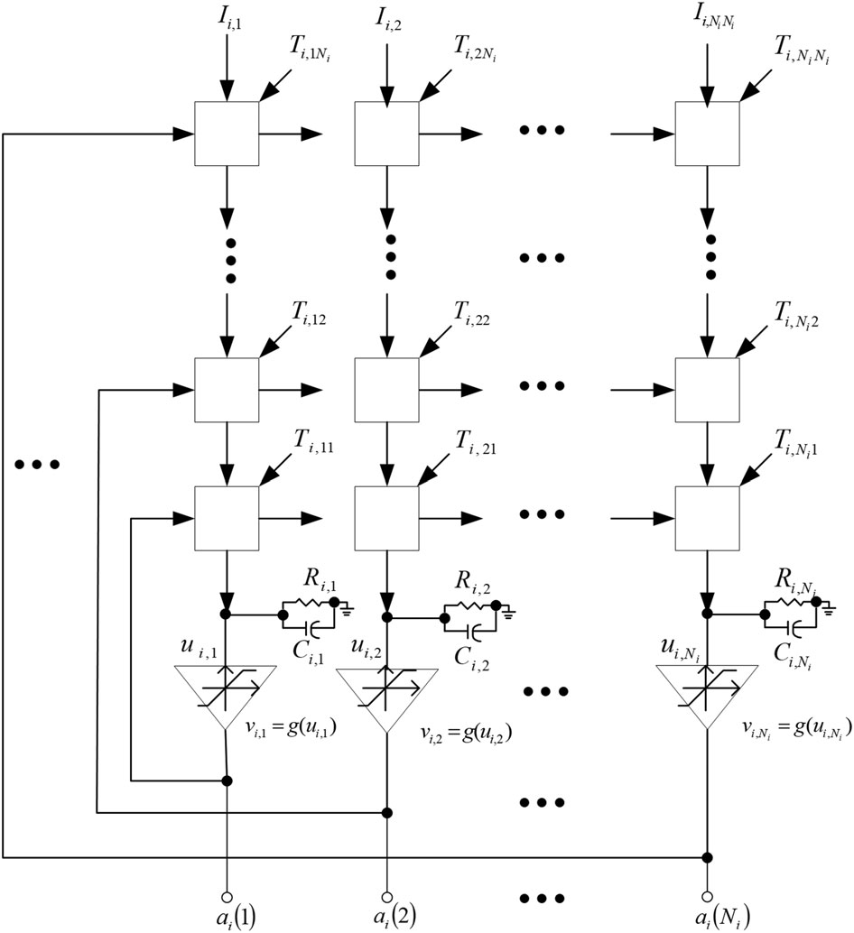
霍普菲尔德神经网络49-52由于具备多种优势，在解决复杂优化问题方面具有强大的潜力。霍普菲尔德神经网络中第 m个神经元的状态动态由非线性微分方程表征，

$$
\frac{du_m}{dt} = -\frac{u_m}{\tau_m} + \sum_{n=1}^{p} T_{mn}v_n + I_m; \tag{22}
$$

其中 τm是与输入电容和电阻相关的时间常数，p为神经元数量，Im为外部输入，Tmn为互连强度。通常，控制输出状态vm与内部状态um关系的S形函数g(um)，其斜率为 λ，表达式如下：

$$
v_m = g(u_m) = \frac{1}{1 + e^{-u_m / \lambda}}: \tag{23}
$$

由于大规模规则互连的神经元结构，该神经网络易于使用模拟超大规模集成电路技术46,50实现。如果待最小化的目标函数能够映射为如下所示的李雅普诺夫能量函数，则霍普菲尔德神经网络可以提供一个理想的解：

$$
E_L = -\frac{1}{2} \sum_{m=1}^{p} \sum_{n=1}^{p} T_{mn} v_m v_n - \sum_{m=1}^{p} I_m v_m + \sum_{m=1}^{p} \frac{1}{\tau_m} \int_{0}^{v_m} g^{-1}(v) dv: \tag{24}
$$

如果等式右侧的第三项不影响优化性能，则可以忽略(22)中的对应项−um/τm ，以提高收敛速度。44,46,52

3.3 | Link o f 霍普菲尔德神经网络和IIR全通型QMF滤波器组设计 n

为了将基于IIR全通的QMF滤波器组的最小二乘设计与李雅普诺夫能量函数相关联，(17)可以展开为

$$
E_i = \sum_{l=1}^{L_i} \sum_{m=1}^{N_i} \sum_{n=1}^{N_i} a_i(m) a_i(n) \sin(\vartheta_{d,i}(\omega_l) - 2m\omega_l) \sin(\vartheta_{d,i}(\omega_l) - 2n\omega_l) \
+ 2\sum_{l=1}^{L_i} \sin(\vartheta_{d,i}(\omega_l)) \sum_{m=1}^{N_i} a_i(m) \sin(\vartheta_{d,i}(\omega_l) - 2m\omega_l) \
+ \sum_{l=1}^{L_i} \sin^2(\vartheta_{d,i}(\omega_l)) \
= \sum_{m=1}^{N_i} \sum_{n=1}^{N_i} a_i(m) a_i(n) \sum_{l=1}^{L_i} \sin(\vartheta_{d,i}(\omega_l) - 2m\omega_l) \sin(\vartheta_{d,i}(\omega_l) - 2n\omega_l) \
+ \sum_{m=1}^{N_i} a_i(m) \sum_{l=1}^{L_i} 2 \sin(\vartheta_{d,i}(\omega_l)) \sin(\vartheta_{d,i}(\omega_l) - 2m\omega_l) \
+ \sum_{l=1}^{L_i} \sin^2(\vartheta_{d,i}(\omega_l)): \tag{25}
$$

显然，常数项 $\sum_{l=1}^{L_i} \sin^2(\vartheta_{d,i}(\omega_l))$可以忽略，因为它与全通滤波器系数无关。因此，基于IIR全通的QMF滤波器组最小二乘设计的Hopfield相关参数可推导为

$$
T_{i,mn} = -\sum_{l=1}^{L_i} \sin(\vartheta_{d,i}(\omega_l) - 2m\omega_l) \sin(\vartheta_{d,i}(\omega_l) - 2n\omega_l): \tag{26}
$$

)

表1比较了不同算法在相关矩阵上所需的计算量。

矩阵 or 向量操作	算法	本文提出	Jou 等人26	Eigenfilter25,32	传统最小二乘法
Qi
加法		(3Li − 1)Ni(Ni+ 1)/2	3(Li − 1)Ni²		3LiNi² − Ni² + 2LiNi − Ni
乘法		2LiNi(Ni+ 1)	4LiNi²		4LiNi² + 2LiNi
三角学		LiNi(Ni+ 1)	2LiNi²		2LiNi² + 2LiNi
Ki
加法		(2Li − 1)Ni	4Ni		12Ni
乘法		2LiNi	12Ni
三角学		LiNi	6Ni
Hi
加法		(3Li − 1)(2Ni − 1)	7(2Ni − 1)		7(2Ni − 1)
乘法		2Li(2Ni − 1)	12(2Ni − 1)		12(2Ni − 1)
三角学		Li(2Ni − 1)	6(2Ni − 1)		6(2Ni − 1)
di
加法		LiNi	12Ni	(2Li − 1)Ni	(2Li − 1)Ni
乘法		3LiNi	24Ni	2LiNi	2LiNi
三角学		2LiNi	6Ni	2LiNi	2LiNi
必需		Ti = −Qi	Qi = Ki + Hi	Qi	Qi
矩阵		Ii = di	di	di	di
总计加法		9LiNi − 3Li − 3Ni + 1	30Ni − 7	(3Li − 1)Ni(Ni + 1)/2	3LiNi² − Ni² + 2LiNi − Ni
乘法		9LiNi − 2Li	60Ni − 12	2LiNi(Ni + 1)	4LiNi² + 2LiNi
三角学		5LiNi − Li	24Ni − 6	LiNi(Ni + 1)	2LiNi² + 2LiNi
滤波器系数		Δai = Ti ai + Ii	(Ki + Hi)ai = di	Qi ai = λmin ai	ai = Qi⁻¹ di
复杂度		O(N²)	O(N²)	O(N³)	O(N³)

Ki 是托普利茨矩阵，Hi 是汉克尔矩阵，λmin 是Qi 的一个变体对应的最小特征值，Li = lNi，l = 3~10，i = 1，2。
Ii;m ¼ À
X
Li
l¼1
sin ϑd;i ð ωlÞ sin ϑd;i ð ωlÞÀ2mωl ; (27)
where 1 ≤ m, n ≤ Ni and pi ¼ Ni, where i ¼ 1, 2 is the number of neurons required to implement the QMF filter bank design.
The all-pass filter coefficients ai(m) correspond to the output states vi,m of the Hopfield neural network, that is, ai(m) ¼ vi,m, for 1 ≤ m ≤
Ni. Obviously, Ti,mn is a real, symmetric, and positive definite matrix; therefore, Ni(Ni þ 1)/2 different elements need to be calculated.
Table 1 compares the computational requirements of different algorithms on the related matrices.
Using trigonometric identities, the interconnection strength Ti,mn can be expanded into a Toeplitz-plus-Hankel matrix form.26,30 Therefore,
3Ni À 1 different elements (Ni and 2Ni À 1 elements required for the Toeplitz and Hankel matrices, respectively) need to be calculated and
stored in the interconnection strength. Obviously, using the characteristics of the Toeplitz-plus-Hankel matrix can significantly reduce the
computational burden compared with only using symmetry. Further adopting the frequency sampling method,26 the calculation of Hopfield
related strengths can be explicitly derived. When the required matrices are determined, the proposed method can obtain the IIR all-pass
filter coefficients with O(N2) complexity, whereas eigenvalue-based and least squares methods require O(N3) complexity.
When applying the Hopfield neural network to realize the least-squares design of the IIR all-pass-based QMF filter bank, two networks
are needed to design the all-pass filter coefficients a1(n) and a2(n). The difference between these two networks lies in the filter orders
(N1, N2) and desired phase responses (θd,1(ω), θd,2(ω)), which can be determined from the Hopfield-related parameters.
The state dynamics of the Hopfield neural network in (22) can be implemented as
Δui;m ¼
P
pi
n¼1 Ti;mnvi;n þ Ii;m
Δt (28)
where Δt is sufficiently small, and ui,m/τi,m is ignored to improve convergence speed.44,46,52 Thus, the input state ui,m of the neural
network at the (t þ 1)th iteration is obtained by the following equation:
ui;m t þ 1 ð Þ ¼ ui;m ð tÞ þ Δui;m; for1≤m≤pi: (29)
Some literature44,46,50,51 indicates that neuron activation functions with non-decreasing characteristics can be used for state dynamics.
Therefore, any neuron with a non-negative slope (dvi,m/dui,m ≥ 0 for 1 ≤ m ≤ pi) can ensure the network converges to a local minimum.
In this paper, neuron activation is approximated by a soft limiter, as shown below
vi;m t þ 1 ð Þ ¼ g ui;m t þ 1 ð Þ ¼
c if ui;m t þ 1 ð Þ≥cλ
ui;m t þ 1 ð Þ
λ if‐cλ<ui;m t þ 1 ð Þ
<

:
(30)
where c determines the dynamic range, and λ controls the convergence speed. Figure 3 shows the Hopfield neural network applied to the
design of IIR all-pass-type QMF filter banks. Figure 4 summarizes the design flow of the proposed neural network technique.
4 | SIMULATION RESULTS AND COMPARISON
In this section, the design of IIR all-pass filters for a two-channel linear-phase QMF filter bank based on the Hopfield neural network is
implemented using the MATLAB software package. To evaluate the design performance of the proposed neural network-based method,
the specifications for the all-pass-type QMF filter bank design are set the same as those of other methods.11,12,15,25,26 Two neural networks
with different numbers of neurons and Hopfield-related parameters are simultaneously designed to obtain the IIR all-pass filters a1(n)
and a2(n). The initial states of the Hopfield neural network are set as ui,m(0) ¼ 10À4, vi,m(0) ¼ 0, and Δt ¼ 10À8, 1 ≤ m ≤ Ni, i ¼
1, 2. The values of the soft limiter are chosen as c ¼ 3 and λ ¼ 400. In the design examples, the frequency sampling grid Li ¼ 8(Ni þ 1),
i ¼ 1, 2 is set within the desired band.
To evaluate the design performance of different methods, the peak stopband ripple (PSR) of H0(ejω), maximum variation of phase
response (MVPR), maximum variation of group delay (MVGD), and maximum variation of QMF filter bank response (MVFBR) are used
for comparison evaluation. These terms are defined as follows15,25,26:
PSR ¼ 20 log10 max
ω∈ ωs;π ½ H0 ej ω
(31)
MVPR ¼ max ω∈½ 0;π Arg M ej ω þ 2N0 þ 2N1 þ 1 ð Þω (32)
MVGD ¼ max ω∈½ 0 ;π GD M ej ω À 2N0 þ 2N1 þ 1 ð Þ (33)
MVFBR ¼ max
ω∈½ 0 ;π 20 log10 M ej ωÀ12e Àj 2N0þ2N1þ1 ð Þω
(34)
where Arg(•) and GD(•) represent the phase response and group delay response, respectively.
Example 1: IIR all-pass filters A1(z2) and A2(z2) with the same order N1 ¼ N2 ¼ 2 (case 1) are designed to satisfy the low-pass analysis
filter H0(z) with passband and stopband edge frequencies of ωp ¼ 0.4π and ωs ¼ 0.6π, respectively. Two Hopfield neural networks (as
shown in Figure 3) run for 5 μs to approximate the convergence of the dynamic states v1,n and v2,n, which correspond to the all-pass filter
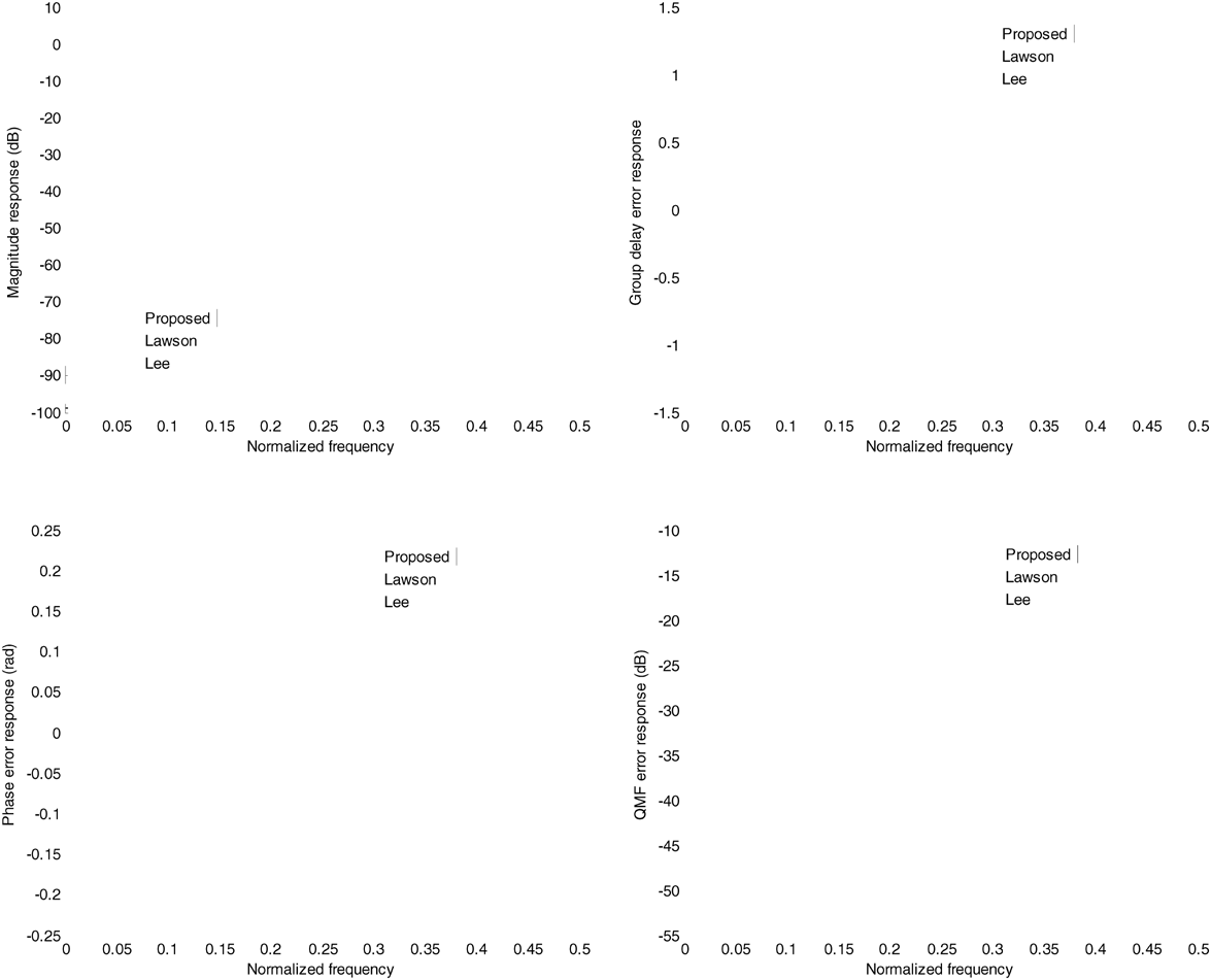
coefficients a1(n) and a2(n), respectively. Figure 5 shows the results designed by the proposed neural network-based method, the Lawson
method, and the Lee–Yang method. Obviously, the magnitude response of the designed analysis filter achieves good low-pass and high-
pass characteristics, as shown in Figure 5A. The proposed method has better stopband attenuation performance than the other methods.
Figure 5B,C shows
FIGURE 3 Design of IIR all-pass-type QMF filter bank based on Hopfield neural network (i ¼ 1, 2)
JOU ET AL.
9
that the proposed neural network-based method has smaller phase error and group delay error responses compared to the other methods.
The magnitude error response of the designed QMF filter bank is superior to the other methods, as can be seen from Figure 5D. Table 2
lists the IIR all-pass filter coefficients designed using different techniques. In this table, an efficient weighted least-squares algorithm that
utilizes the Toeplitz-plus-Hankel matrix for IIR all-pass filter design is also included.
Figure 4 Design flow of IIR all-pass-type QMF filter bank using neural network
10
JOU ET AL.
that the proposed neural network-based method has smaller phase error and group delay error responses compared to the other methods.
The magnitude error response of the designed QMF filter bank is superior to the other methods, as can be seen from Figure 5D. Table 2
lists the IIR all-pass filter coefficients designed using different techniques. In this table, an efficient weighted least-squares algorithm that
utilizes the Toeplitz-plus-Hankel matrix for IIR all-pass filter design is also included.
Figure 4 Design flow of IIR all-pass-type QMF filter bank using neural network
10
JOU ET AL.
Comparison results show that the filter coefficients obtained by the proposed Hopfield neural network are very close to the results of the
literature methods. Since there is no significant difference in design accuracy compared to Jou et al.26 and Kidambi’s method,30 the
corresponding curves of these methods26,30 are omitted in Figure 5.
Example 2: IIR all-pass filters A1(z2) and A2(z2) with orders N1 ¼ 3 and N2 ¼ 2, respectively (case 2), are designed to satisfy the low-
pass analysis filter H0(z) with passband and stopband edge frequencies of ωp ¼ 0.4π and ωs ¼ 0.6π, respectively. The proposed neural
network-based method outperforms the Lee and Yang method15 in terms of stopband attenuation but is slightly less accurate than other
methods.12 Figure 6A shows the magnitude response of the designed filters
FIGURE 5 Design results of Example 1. A, Magnitude response of analysis filters. B, Phase error response. C, Group delay error response. D,
Magnitude error response of QMF design [Color figure can be viewed at wileyonlinelibrary.com]
TABLE 2 IIR All-Pass Filter Coefficients Design for Example 1
a1(n)
n Proposed Kidambi30(Jou et al.26) Lawson11 Lee and Yang15
0 1.00000000000000 1.00000000000000 1.00000000000000 1.00000000000000
1 À0.22275012748626 À0.22275018664134 À0.23192007497764 À0.23721170339174
2 0.10285224508044 0.10285230782734 0.09293506470691 0.15616284195027
a2(n)
n Proposed Kidambi30(Jou et al.26) Lawson11 Lee and Yang15
0 1.00000000000000 1.00000000000000 1.00000000000000 1.00000000000000
1 0.23053244219645 0.23053250202522 0.23192007497764 0.23401447596825
2 À 0.06203533601293 À 0.06203545095846 À 0.09293506470690 À 0.09173259794723
JOU ET AL.
11
low-pass and high-pass analysis filters. From Figure 6B,C, it can be seen that the proposed neural network-based method performs better
in phase and group delay responses than the Lawson and Klouche-Djedid12 and Lee–Yang15 methods. Figure 6D shows the comparison
of the magnitude error response of the QMF filter bank. Obviously, in most frequency bands, the magnitude error response produced by
the proposed neural network-based method is smaller than the results of the Lawson and Klouche-Djedid12 and Lee–Yang15 methods. The
proposed neural network-based method almost achieves the same effect
FIGURE 6 Design results of Example 2. A, Magnitude response of analysis filters. B, Phase error response. C, Group delay error response. D,
Magnitude error response of QMF design [Color figure can be viewed at wileyonlinelibrary.com]
TABLE 3 IIR All-Pass Filter Coefficients Design for Example 2
a1(n)
n Proposed Kidambi30(Jou et al.26) Lawson and Klouche-Djedid12 Lee and Yang15
0 1.00000000000000 1.00000000000000 1.00000000000000 1.00000000000000
1 0.23514357134253 0.23514388080649 0.23192007497764 0.23809492090228
2 À0.06944063991209 À0.06944116945502 À0.09293506470691 À0.07300653565757
3 0.02504743245405 0.02504803279377 0.04145970439782 0.03862697338297
a2(n)
n Proposed Kidambi30(Jou et al.26) Lawson and Klouche-Djedid12 Lee and Yang15
0 1.00000000000000 1.00000000000000 1.00000000000000 1.00000000000000
1 À0.22275012748626 À0.22275018664134 À0.23192007497764 À0.23721170338893
2 0.10285224508044 0.10285230782734 0.09293506470691 0.15616284193843
12
JOU ET AL.
that the proposed neural network-based method almost achieves the same effect
as Jou et al.26 and Kidambi’s method.30 The IIR all-pass filter coefficients designed using various methods12,15,26,30 are listed in Table 3.
It is worth noting that the explicit formula of the Lawson algorithm11,12 yields IIR all-pass filter coefficients with opposite signs, that is,
a2(n) ¼ À a1(n), 1 ≤ n ≤ Ni, i ¼ 1, 2. The relationship between A0(z2) and A1(z2) limits the design flexibility and achievable accuracy.
Therefore, the design results of the Lawson algorithm11,12 lead to larger phase errors and magnitude error responses, as shown in Figures 5
and 6.
The design results using different techniques are summarized in Table 4. Obviously, the values of MVGD and MVPR are better than
those of methods,11,12,15 and are close to the eigenfilter method. The values of PSR and MVFBR are better than or comparable to the
Lawson method. The proposed neural network-based method precisely achieves the same performance level as Jou et al. and Kidambi’s
methods. This can be seen from Tables 2 and 3: the designed IIR all-pass filter coefficients have excellent consistency among the
proposed neural network-based method, Jou et al., and Kidambi’s methods. Simulation results verify that the proposed method performs
better than other methods in both phase and group delay responses. Compared with the eigenfilter-based method, the proposed method
almost achieves the same accuracy. Therefore, the Hopfield neural network can accurately design IIR all-pass-based QMF filter banks
with high performance and large-scale parallelism.
After designing the IIR all-pass filters, low-pass and high-pass analysis filters can be implemented using (3) and (4), thus constituting the
basic building blocks of the two-channel QMF filter bank. Furthermore, combining tree-structured methods or cosine-modulated filter
banks,5 the proposed technique can be easily applied to the design of multichannel filter banks.
5 | CONCLUSION
This study extends a simplified approach using a feedback neural network to design two-channel linear-phase quadrature mirror filter
banks based on IIR all-pass filters. Simulation results verify that the proposed neural network-based method can achieve good phase and
group delay response performance in a parallel structure without introducing amplitude distortion. By appropriately selecting Hopfield-
related parameters, IIR all-pass filter coefficients can be obtained through dynamic nonlinear equations. When the network reaches
convergence, the output states of the neural network approach the optimal IIR all-pass filters. Furthermore, by utilizing the parallel
combination of the designed IIR all-pass filters, complete reconstruction of the two-channel quadrature mirror filter bank can be
achieved. The proposed neural network-based technique can be easily applied to the design of multichannel filter banks by combining
tree-structured methods or cosine-modulated filter banks.
TABLE 4 Comparison of Design Performance with Different Methods
Example Algorithm PSR (dB) MVPR (rad) MVGD (samples) MVFBR (dB)
N1 ¼ 2
N2 ¼ 2
Lawson11 À15.9640 0.1984 1.2139 À20.0857
Lee and Yang15 À18.1039 0.1328 0.8991 À23.5610
Chen et al25 À14.2535 0.1101 0.6984 À25.1859
Jou et al.26 À14.2571 0.1128 0.7122 À24.9792
Kidambi30 À14.2571 0.1128 0.7122 À24.9792
Tkacenko et al.32 À14.2934 0.1122 0.7100 À25.0283
Proposed À14.2571 0.1128 0.7122 À24.9792
N1 ¼ 3
N2 ¼ 2
Lawson and Klouche-Djedid12 À19.1003 0.3028 2.1609 À16.4320
Lee and Yang15 À20.8760 0.2060 1.4980 À19.7606
Chen et al.25 À16.8308 0.2047 1.4085 À19.8120
Jou et al.26 À16.6958 0.2023 1.3873 À19.9139
Kidambi30 À16.6959 0.2023 1.3873 À19.9138
Tkacenko et al.32 À16.7372 0.2015 1.3840 À19.9511
Proposed À16.6958 0.2023 1.3873 À19.9139
JOU ET AL.
13