全连接神经网络实战——AQI空气质量预测

最近在学习深度学习有关的知识，这里记录一个实战练习，供自己理解学习，也提供给大家学习。这里我用的工具是VSCode，数据集可以自己到网站爬取清洗到数据库下载，这个是公开的，也没有什么反爬机制。当然了，考虑到方便小伙伴们的学习，大家可以自行下载我爬取到的数据集~

https://download.youkuaiyun.com/download/luoying189/92265792?spm=1001.2014.3001.5503

话不多说，我们开始实战。

一、数据的预处理

新建py文件：aqi_train.ipynb

1、导入需要的包

import numpy as np

import pandas as pd

import matplotlib.pyplot as plt

from sklearn.preprocessing import MinMaxScaler

from sklearn.model_selection import train_test_split

import keras

from keras .layers import Dense

from tensorflow.python.keras.utils.np_utils import to_categorical

from sklearn.metrics import classification_report

plt.rcParams['font.sans-serif']=['SimHei']  # 用来正常显示中文标签

plt.rcParams['axes.unicode_minus']=False  # 用来正常显示负号

import warnings

warnings.filterwarnings("ignore")

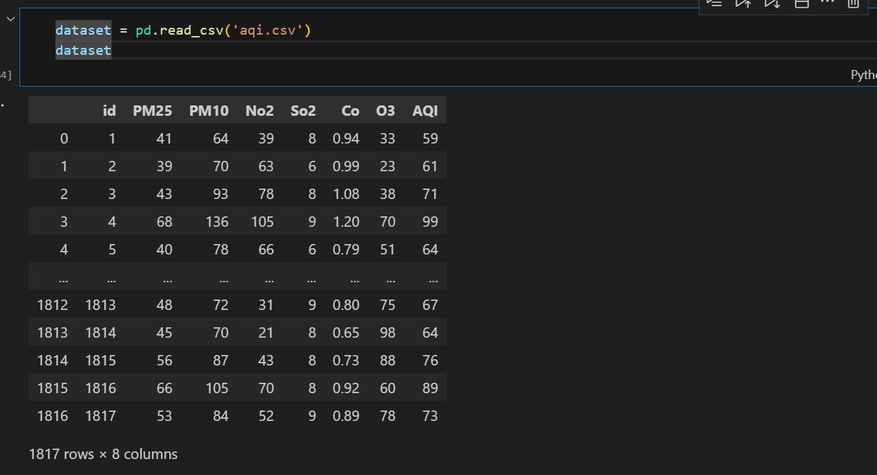
2、导入数据集，可以看到我们的数据集有6个特征，1个标签（AQI）

dataset = pd.read_csv('aqi.csv')

dataset

3、划分特征与标签

X = dataset.iloc[:,1:-1]

Y = dataset['AQI']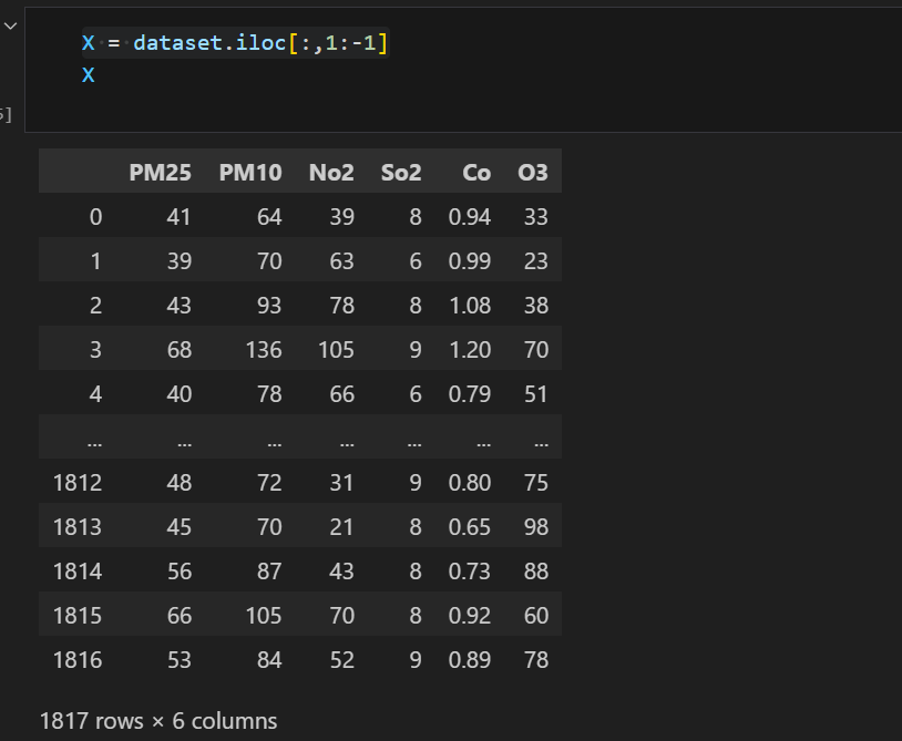

4、划分训练集和测试集，这里我们划分为8：2

x_train,x_test,y_train,y_test = train_test_split(X,Y,test_size=0.2,random_state=42)

5、将数据进行归一化，为什么要进行数据的归一化呢？归一化的核心目的是让所有特征处于同一“量纲”或“尺度”上，从而保证模型能够公平、高效地学习。

举个小例子：

当我们预测房价的时候，特征A:房间面积：90-250平方米，特征B:房间数量1-6个。这两个特征的数值范围相差巨大。如果不进行归一化，模型（尤其是基于距离的算法如KNN、SVM，或使用梯度下降的算法）会认为“房间面积”这个特征因为数值更大，所以更重要，给予的权重也会更大。这显然是不合理的，因为房间数量同样是一个重要的预测因素。

比如，你会买一个200平方米但是只有一个房间的房子吗？大部分人不会买吧？这种房子显然在房子市场不那么受欢迎（当然也不是那么绝对，只是大部分人不会选择，如果我发财了我也会买大房子自己住的~~），但是如果不给予合适权重，就会因为面积大而被刻板标榜高价。

# 数据归一化

sc = MinMaxScaler(feature_range=(0,1))

x_train = sc.fit_transform(x_train)

x_test = sc.transform(x_test)

y_train = pd.DataFrame(y_train)

y_train = sc.fit_transform(y_train)

y_test = pd.DataFrame(y_test)

y_test = sc.transform(y_test)

x_train = x_train.reshape(-1, x_train.shape[-1])   # 或 .values.reshape(-1, n_features)

x_test  = x_test.reshape(-1, x_test.shape[-1])

y_train = y_train.reshape(-1, 1)

y_test  = y_test.reshape(-1, 1)

二、模型建立与训练

1、模型建立，我们添加两个隐藏层，激活函数选择“relu”，由于并不是分类任务，所以输出层输出单个数值就好。

model = keras.Sequential()

model.add(Dense(10,activation='relu'))

model.add(Dense(10,activation='relu'))

model.add(Dense(1))

2、模型编译

model.compile(loss='mse',optimizer='SGD') #SGC随机梯度

3、模型训练，我们训练100轮次，最后保存我们的模型，为了后面的检测

history = model.fit(x_train,y_train,epochs=100,batch_size=24,verbose=2,validation_data=(x_test,y_test))

model.save('aqi_model.keras')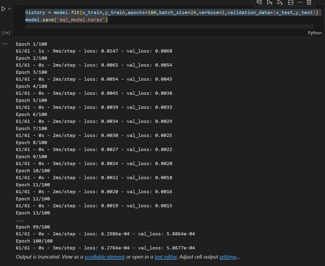

三、模型损失值的可视化

plt.plot(history.history['loss'],label='train')

plt.plot(history.history['val_loss'],label='val')

plt.title('全连接神经网络loss值图')

plt.legend()

plt.show()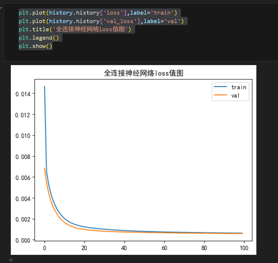

四、模型检测

再新建一个aqi_test.ipynb，前面的步骤其实和aqi_train的代码差不多，你们直接粘贴文件来改也是可以的

1、导包

import numpy as np

import pandas as pd

import matplotlib.pyplot as plt

from sklearn.preprocessing import MinMaxScaler

from sklearn.model_selection import train_test_split

# import keras

# from keras .layers import Dense

from tensorflow.python.keras.utils.np_utils import to_categorical

from sklearn.metrics import classification_report

plt.rcParams['font.sans-serif']=['SimHei']  # 用来正常显示中文标签

plt.rcParams['axes.unicode_minus']=False  # 用来正常显示负号

import warnings

warnings.filterwarnings("ignore")

from sklearn.metrics import mean_squared_error

from keras.models import load_model

from tensorflow import concat as concatenate   # TF 风格

2、导入数据集

dataset = pd.read_csv('aqi.csv')

dataset

3、划分特征与标签

X = dataset.iloc[:,1:-1]

Y = dataset['AQI']

4、划分训练集和测试集，这里我们划分为8：2

x_train,x_test,y_train,y_test = train_test_split(X,Y,test_size=0.2,random_state=42)

5、数据归一化（这里就不太一样了，一起归一化的话不太好）

x_scaler = MinMaxScaler()

y_scaler = MinMaxScaler()

x_train = x_scaler.fit_transform(x_train)

x_test  = x_scaler.transform(x_test)

y_train = y_scaler.fit_transform(y_train.values.reshape(-1, 1))

y_test  = y_scaler.transform(y_test.values.reshape(-1, 1))

6、导入训练好的模型

model = load_model('aqi_model.keras')

7、将数据反归一化，先出来模型预测结果，然后把模型结果反归一化，因为你之前把数据归一化为了范围0-1的数据，但是我们与真实数据进行比较的时候是要用归一化之前的正常值的，所以这里我们要进行反归一化的操作。

yhat = model.predict(x_test)

inv_yhat = y_scaler.inverse_transform(yhat)

# 反向缩放真实值

inv_y = y_scaler.inverse_transform(y_test)

inv_y

8、模型评估，这里就要用均方误差了，可以看到均方误差大约为3.08，这样看我们的模型效果还是蛮不错的

import math

rmse = math.sqrt(mean_squared_error(inv_y,inv_yhat))

mape = np.mean(np.abs(inv_y - inv_yhat)/inv_yhat)

print('rmse',rmse)

print('mape',mape)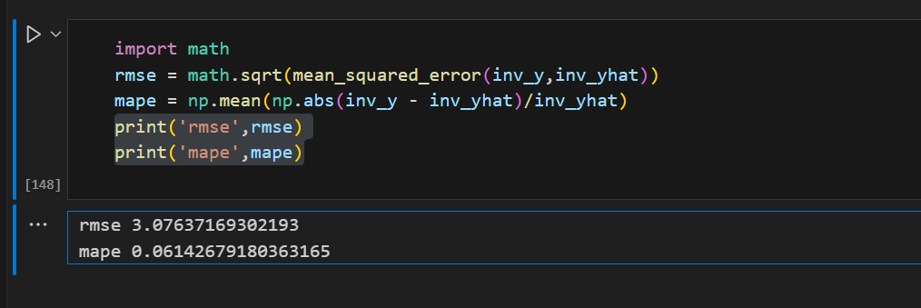

最后可视化一下，看看真实值和预测值的

plt.plot(inv_yhat,label='预测值')

plt.plot(inv_y,label='真实值')

plt.title('对比图')

plt.legend()

plt.show()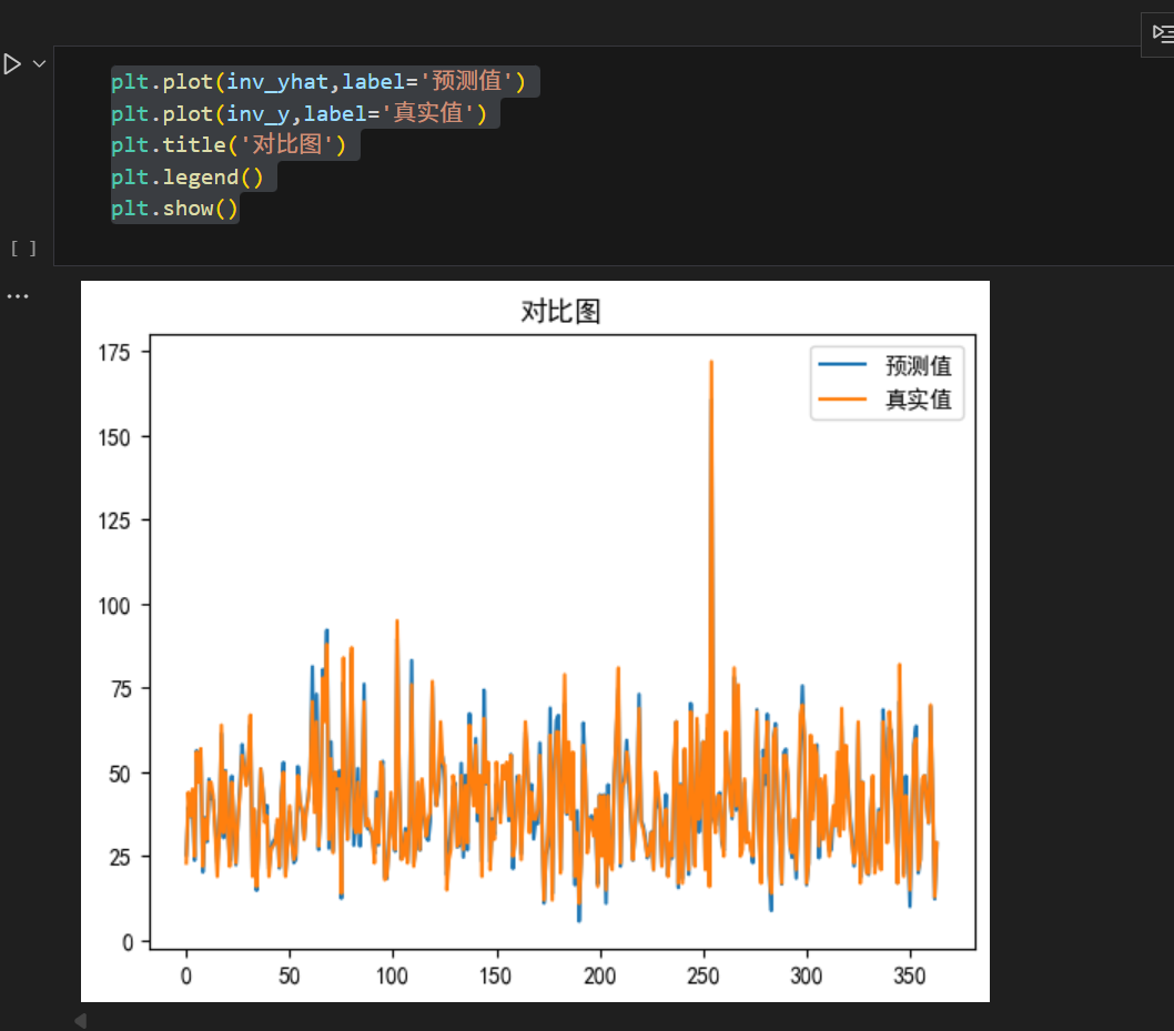

整个全连接神经网络的AQI实战到这里就结束了，需要全部代码的可以看看我的资源，放有完整的代码。

结束，完结撒花~