深度学习：前向传播与反向传播公式推导-优快云博客

1 定义网络结构

假设某二分类问题的网络结构由如图1.1组成（暂仅以2层网络举例，更高层数可依此类比），其输入的特征向量维数为n，隐藏层神经元个数为 $n^{[1]}$ ，输出层神经元个数为 $n^{[2]}$ （由于是二分类问题，故仅含一个）。

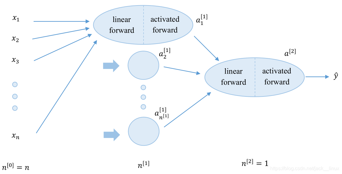
其训练过程为：首先获取训练数据 X ，初始化每层的训练参数 w、b ，并通过前向传播算法（包含线性前向传播和激活函数前向传播）得到 $\hat y$ 并计算 $J(w,b)$ ，然后通过反向传播算法（包含线性反向传播和激活函数反向传播）计算每层的 dw 和 db，最终通过梯度下降算法更新参数 w、b，并多次迭代该过程，得到训练参数。

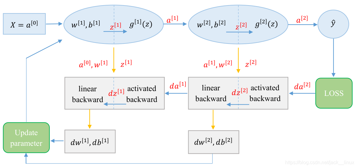
其中参数为：

$X = \begin{bmatrix} X_1^{(1)} X_1^{(2)} ... \ X_1^{(m)} \\ X_2^{(1)} X_2^{(2)} ... \ X_2^{(m)} \\ ... ... ... ... \\ X_{n^{[0]}}^{(1)} X_{n^{[0]}}^{(2)} ... \ X_{n^{[0]}}^{(m)} \end{bmatrix}_{(n^{[0]}\times m)}$ $W^{[1]T} = \begin{bmatrix} W_{11}^{[1]} \ \ W_{12}^{[1]} \ ... \ W_{1n^{[0]}}^{[1]} \\ W_{21}^{[1]} \ \ W_{22}^{[1]} ... \ W_{2n^{[0]}}^{[1]} \\ ... ... ... ... \\ W_{n^{[1]}1}^{[1]} W_{n^{[1]}2}^{[1]} ... \ W_{n^{[1]}n^{[0]}}^{[1]} \end{bmatrix}_{(n^{[1]}\times n^{[0]})}$ $b^{[1]} = \begin{bmatrix} b_{1}^{[1]} \\ b_{2}^{[1]}\\ ... \\ b_{n^{[1]}}^{[1]} \end{bmatrix}_{(n^{[1]}\times 1)}$

类比可知 $W^{[2]T}$ 维数为 $(n^{[2]} \times n^{[1]})$ ， $b^{[2]}$ 维数为 $(n^{[2]} \times 1)$ 。

X 包含 m 个样本的 $n^{[0]}$ 个特征值， $W^{[1]}$ 包含网络第1层的所有权重参数， $b^{[1]}$ 包含网络第1层的所有偏置参数。

2 前向传播算法

输入数据 X ，然后通过每层的权重 w 和偏置 b 计算得到输出预测值 $\hat y$ ，并最终通过代价函数衡量算法的运行情况。

$Z^{[1]} =W^{[1]T}X + b^{[1]}= \begin{bmatrix} Z_{1}^{[1](1)} \ Z_{1}^{[1](2)} \ ... \ Z_{1}^{[1](m)} \\ Z_{2}^{[1](1)} \ Z_{2}^{[1](2)} ... \ Z_{2}^{[1](m)} \\ ... ... ... ... \\ Z_{n^{[1]}}^{[1](1)} Z_{n^{[1]}}^{[1](2)} ... \ \ Z_{n^{[1]}}^{[1](m)} \end{bmatrix}_{(n^{[1]}\times m)}$

注：上式中 ${\color{Red} b^{[1]}}$ 需要先广播（python中的一种运算机制）至 ${\color{Red} (n^{[1]} \times m)}$ 再参与运算。

$A^{[1]}=g^{[1]}(Z^{[1]})$ ，此处激活函数 $g^{[1]}(z)$ 选择 Relu 函数。

$Z^{[2]} =W^{[2]T}A^{[1]} + b^{[2]}$

$A^{[2]}=g^{[2]}(Z^{[2]})$ ，此处激活函数 $g^{[2]}(z)$ 选择 sigmoid 函数。

$\hat y=A^{[2]}$ ，即为输出的预测值。

损失函数： $L(\hat y,y)=-ylog(\hat y)-(1-y)log(1-\hat y)$

代价函数（暂不考虑正则化）： $J(w,b)=\frac {1}{m} \sum_{i=1}^m L(\hat y,y)$

注意：此处不同于线性回归的平方和代价函数，因为sigmoid函数在平方和函数（ $J(w,b)=\frac {1}{m} \sum_{i=1}^m \frac{1}{2}(\hat y-y)^2$ ）中会成为“非凸函数”，产生很多局部最小值，这对后续的梯度下降法寻找最优值是极为不利的，故重此处新定义代价函数。

3 反向传播算法

可以说，一个神经网络的计算，都是按照前向或反向传播过程组织的。首先我们计算出一个新的网络的输出（前向过程），紧接着进行一个反向传输操作。后者即用来计算出每层神经元对应的梯度或导数。

3.1计算图

如图3.1，先举一个计算图的例子，该例也可从本质上反应反向传播算法的计算过程。

此处先对 $v$ 求导， $\frac {dJ}{dv}=3$

接下来向前传递一次， $\frac {dJ}{du}=\frac {dJ}{dv}\frac {dv}{du}=3*1=3$

即可得到 a, b, c 的所有导数：

$\frac {dJ}{da}=\frac {dJ}{dv}\frac {dv}{da}=3*1=3$

$\frac {dJ}{db}=\frac {dJ}{dv}\frac {dv}{du}\frac {du}{db}=3*1*c=6$

$\frac {dJ}{dc}=\frac {dJ}{dv}\frac {dv}{du}\frac {du}{dc}=3*1*b=9$

3.2 反向传播

该例为一简易的逻辑回归，其计算图如图3.2所示（代码中我们使用dx表示变量x的导数）：

(1) 因为 $da^{[2]} =\frac {\partial J(w,b)} {\partial a^{[2]}}$ 且 $J(w,b) = \frac {1}{m} \sum_{i=1}^mL(\hat y,y)$ ，输出值 $\hat y = a^{[2]}$ ，故 $da^{[2]} = \frac {1}{m} \sum_{i=1}^m \frac{\partial L(a^{[2]},y)}{\partial a^{[2]}} = \frac{\partial L(a^{[2]},y)}{\partial a^{[2]}}$

又因为，在逻辑回归中，损失函数 $L(a,y) = -ylog(a)-(1-y)log(1-a)$

故 ${\color{Blue} da^{[2]}=\frac{\partial L(a,y)}{\partial a^{[2]}} = \frac {-y}{a^{[2]}} + \frac{1-y}{1-a^{[2]}}}$

(2) 根据计算图向前计算一步， $dz^{[2]} =\frac{\partial L(a,y)}{\partial a^{[2]}}\frac{\partial a^{[2]}}{\partial z^{[2]}}= da^{[2]} * g^{[2]'}(z^{[2]})$

因为 $g^{[2]}(z)=\frac{1}{1+e^{-z}}$ ，故其导函数

$g^{'}(z) = -\frac {1}{(1+e^{-z})^2} * e^{-z} * (-1) = \frac {e^{-z}}{(1+e^{-z})^2} = \frac {1}{1+e^{-z}} * (1-\frac{1}{1+e^{-z}}) = g(z) * (1-g(z))$

因为 $a=g(z)$ ，故 $g^{'}(z) = a * (1-a)$

则 ${\color{Blue} dz^{[2]} =(\frac {-y}{a^{[2]}} + \frac {1-y}{1-a^{[2]}}) * a^{[2]}(1-a^{[2]}) = a^{[2]}-y}$

(3) 根据计算图，再次推进一步， $dw^{[2]} =\frac {\partial J(w,b)} {\partial w^{[2]}}=\frac {\partial J(w,b)} {\partial a^{[2]}}\frac{\partial a^{[2]}}{\partial z^{[2]}}\frac{\partial z^{[2]}}{\partial w^{[2]}}=dz^{[2]} \frac{\partial z^{[2]}}{\partial w^{[2]}}$

因为 $\frac{\partial z^{[2]}}{\partial w^{[2]}}=a^{[1]T}$ ，故 ${\color{Blue} dw^{[2]} =dz^{[2]}*a^{[1]T}}$

(4) $db^{[2]} =\frac {\partial J(w,b)} {\partial b^{[2]}}=\frac {\partial J(w,b)} {\partial a^{[2]}}\frac{\partial a^{[2]}}{\partial z^{[2]}}\frac{\partial z^{[2]}}{\partial b^{[2]}}=dz^{[2]} \frac{\partial z^{[2]}}{\partial b^{[2]}}$

因为 $\frac{\partial z^{[2]}}{\partial b^{[2]}}=1$ ，故 ${\color{Blue} db^{[2]} =dz^{[2]}}$

(5) $da^{[1]} =\frac {\partial J(w,b)} {\partial a^{[1]}}=\frac {\partial J(w,b)} {\partial a^{[2]}}\frac{\partial a^{[2]}}{\partial z^{[2]}}\frac{\partial z^{[2]}}{\partial a^{[1]}}=dz^{[2]} \frac{\partial z^{[2]}}{\partial a^{[1]}}$

因为 $\frac{\partial z^{[2]}}{\partial a^{[1]}}=w^{[2]T}$ ，故 ${\color{Blue} da^{[1]} =dz^{[2]}*w^{[2]T}}$

(6) $dz^{[1]} =\frac {\partial J(w,b)} {\partial z^{[1]}}=\frac {\partial J(w,b)} {\partial a^{[2]}}\frac{\partial a^{[2]}}{\partial z^{[2]}}\frac{\partial z^{[2]}}{\partial a^{[1]}}\frac{\partial a^{[1]}}{\partial z^{[1]}}=da^{[1]} \frac{\partial a^{[1]}}{\partial z^{[1]}}$

因为 $\frac{\partial a^{[1]}}{\partial z^{[1]}}=g^{[1]'}(z^{[1]})$ ，故 ${\color{Blue} dz^{[1]} =da^{[1]}*g^{[1]'}(z^{[1]})}$

(7) $dw^{[1]} =\frac {\partial J(w,b)} {\partial z^{[1]}}=\frac {\partial J(w,b)} {\partial a^{[2]}}\frac{\partial a^{[2]}}{\partial z^{[2]}}\frac{\partial z^{[2]}}{\partial a^{[1]}}\frac{\partial a^{[1]}}{\partial z^{[1]}}\frac{\partial z^{[1]}}{\partial w^{[1]}}=dz^{[1]} \frac{\partial z^{[1]}}{\partial w^{[1]}}$

因为 $\frac{\partial z^{[1]}}{\partial w^{[1]}}=X^T$ ，故 ${\color{Blue} dw^{[1]} =dz^{[1]}*X^T}$

(8) $db^{[1]} =\frac {\partial J(w,b)} {\partial z^{[1]}}=\frac {\partial J(w,b)} {\partial a^{[2]}}\frac{\partial a^{[2]}}{\partial z^{[2]}}\frac{\partial z^{[2]}}{\partial a^{[1]}}\frac{\partial a^{[1]}}{\partial z^{[1]}}\frac{\partial z^{[1]}}{\partial b^{[1]}}=dz^{[1]} \frac{\partial z^{[1]}}{\partial b^{[1]}}$

因为 $\frac{\partial z^{[1]}}{\partial b^{[1]}}=1$ ，故 ${\color{Blue} db^{[1]} =dz^{[1]}}$

注意：由于X是固定的，且所有所需的参数dw、db也已全部求导完成，也不需要对X进行优化，故不需要对 $da^{[0]}$ 进行求导。

至此，反向传播算法的所有计算步骤已全部推导完成，接下来只需将计算式向量化为代码所需的形式即可。

3.3 向量化

对应上述所有计算式，向量化为：

(1) ${\color{Blue} dZ^{[2]}=A^{[2]}-Y}$

(2) ${\color{Blue} dW^{[2]} =\frac{1}{m}dZ^{[2]}*A^{[1]T}}$ （注意：其中加入 ${\color{Red} \frac{1}{m}}$ 求平均是因为防止样本过大而导致数值过大的情况）

(3) ${\color{Blue} db^{[2]} =\frac{1}{m}np.sum(dZ^{[2]},axis=1,keepdims=True)}$

(4) ${\color{Blue} dZ^{[1]}=W^{[2]T}dZ^{[2]}*g^{[1]'}(Z^{[1]})}$

(5) ${\color{Blue} dW^{[1]} =\frac{1}{m}dZ^{[1]}*X^{[1]T}}$

(6) ${\color{Blue} db^{[1]} =\frac{1}{m}np.sum(dZ^{[1]},axis=1,keepdims=True)}$

4 梯度下降算法

梯度下降是一个用来求函数最小值的算法，此处将使用梯度下降算法来求出代价函数 $J(w,b)$ 的最小值。梯度下降背后的思想是：开始时随机初始化参数w、b，并通过前向传播计算代价函数，然后寻找下一个能让代价函数值下降最多的参数组合。多次迭代该步骤直到找到一个局部最小值。

梯度下降算法的种类较多，此处仅以批量梯度下降算法为例，其公式为：

repeat until convergence{

$w=w-a\frac{\partial }{\partial w}J(w,b)$

$b=b-a\frac{\partial }{\partial b}J(w,b)$

}

其中 a 是学习率（learning rate），它决定了我们沿着能让代价函数下降程度最大的方向向下迈出的步子有多大。

5 代码实现

import neural_networks as nn

n0 = train_x.shape[0]             # 输入的特征向量维数：12288
Layer = (n0, 20, 7, 5, 1)         # 定义4层网络，3个隐藏层，1个输出层

parameters = nn.L_layer_model(train_x, train_y, Layer, num_iterations = 2500, print_cost = True)    # 执行该函数后即可得到优化后的参数w、b

import numpy as np

def initialize_parameters_deep(layer_dims):
    np.random.seed(1)
    parameters = {}
    L = len(layer_dims)            # number of layers in the network

    for l in range(1, L):
        parameters['W' + str(l)] = np.random.randn(layer_dims[l], layer_dims[l-1]) * np.sqrt(1 / layer_dims[l-1]) # * 0.01
        parameters['b' + str(l)] = np.zeros((layer_dims[l], 1))
        
        assert(parameters['W' + str(l)].shape == (layer_dims[l], layer_dims[l-1]))
        assert(parameters['b' + str(l)].shape == (layer_dims[l], 1))

    return parameters

"""
Implements the sigmoid activation in numpy
"""
def sigmoid(Z):

    A = 1/(1+np.exp(-Z))
    cache = Z
    
    return A, cache

"""
Implement the RELU function.
"""
def relu(Z):

    A = np.maximum(0,Z)
    
    assert(A.shape == Z.shape)
    
    cache = Z 
    return A, cache


"""
Implement the backward propagation for a single RELU unit.
"""
def relu_backward(dA, cache):

    Z = cache
    dZ = np.array(dA, copy=True) # just converting dz to a correct object.
    
    # When z <= 0, you should set dz to 0 as well. 
    dZ[Z <= 0] = 0
    
    assert (dZ.shape == Z.shape)
    
    return dZ


"""
Implement the backward propagation for a single SIGMOID unit.
"""
def sigmoid_backward(dA, cache):

    Z = cache
    
    s = 1/(1+np.exp(-Z))
    dZ = dA * s * (1-s)
    
    assert (dZ.shape == Z.shape)
    
    return dZ

"""
Implement the linear part of a layer's forward propagation.
"""
def linear_forward(A, W, b):

    Z = np.dot(W, A) + b
    
    assert(Z.shape == (W.shape[0], A.shape[1]))
    cache = (A, W, b)
    
    return Z, cache


"""
Implement the forward propagation for the LINEAR->ACTIVATION layer
"""
def linear_activation_forward(A_prev, W, b, activation):
    if activation == "sigmoid":
        # Inputs: "A_prev, W, b". Outputs: "A, activation_cache".
        Z, linear_cache = linear_forward(A_prev, W, b)
        A, activation_cache = sigmoid(Z)
    elif activation == "relu":
        # Inputs: "A_prev, W, b". Outputs: "A, activation_cache".
        Z, linear_cache = linear_forward(A_prev, W, b)
        A, activation_cache = relu(Z)
    
    assert (A.shape == (W.shape[0], A_prev.shape[1]))
    cache = (linear_cache, activation_cache)

    return A, cache

"""
Implement forward propagation for the [LINEAR->RELU]*(L-1)->LINEAR->SIGMOID computation
"""
def L_model_forward(X, parameters):
    caches = []
    A = X
    L = len(parameters) // 2                  # number of layers in the neural network
    
    # Implement [LINEAR -> RELU]*(L-1). Add "cache" to the "caches" list.
    for l in range(1, L):
        A_prev = A 
        A, cache = linear_activation_forward(A_prev, parameters['W' + str(l)], \
            parameters['b' + str(l)], activation = "relu")
        caches.append(cache)
    
    # Implement LINEAR -> SIGMOID. Add "cache" to the "caches" list.
    AL, cache = linear_activation_forward(A, parameters['W' + str(L)], \
            parameters['b' + str(L)], activation = "sigmoid")
    caches.append(cache)
    
    assert(AL.shape == (1,X.shape[1]))
            
    return AL, caches

"""
Implement the cost function defined by equation (7).
"""
def compute_cost(AL, Y):
    m = Y.shape[1]

    # Compute loss from aL and y.
    cost = (1./m) * (-np.dot(Y,np.log(AL).T) - np.dot(1-Y, np.log(1-AL).T))
    cost = np.squeeze(cost)      # To make sure your cost's shape is what we expect (e.g. this turns [[17]] into 17).
    assert(cost.shape == ())
    
    return cost


"""
Implement the linear portion of backward propagation for a single layer (layer l)
"""
def linear_backward(dZ, cache):
    
    A_prev, W, b = cache  # b没用上
    m = A_prev.shape[1]
    
    dW = (1 / m) * np.dot(dZ, A_prev.T)
    db = (1 / m) * np.sum(dZ, axis=1, keepdims=True)
    dA_prev = np.dot(W.T, dZ)
    
    assert (dA_prev.shape == A_prev.shape)
    assert (dW.shape == W.shape)
    assert (db.shape == b.shape)
    
    return dA_prev, dW, db


"""
Implement the backward propagation for the LINEAR->ACTIVATION layer.
"""
def linear_activation_backward(dA, cache, activation):
    
    linear_cache, activation_cache = cache
    
    if activation == "relu":
        dZ = relu_backward(dA, activation_cache)
        dA_prev, dW, db = linear_backward(dZ, linear_cache)
        
    elif activation == "sigmoid":
        dZ = sigmoid_backward(dA, activation_cache)
        dA_prev, dW, db = linear_backward(dZ, linear_cache)
    
    return dA_prev, dW, db


"""
Implement the backward propagation for the [LINEAR->RELU] * (L-1) -> LINEAR -> SIGMOID group
"""
def L_model_backward(AL, Y, caches):
    
    grads = {}
    L = len(caches) # the number of layers
#    m = AL.shape[1]
    Y = Y.reshape(AL.shape) # after this line, Y is the same shape as AL

    # Initializing the backpropagation
    dAL = - (np.divide(Y, AL) - np.divide(1 - Y, 1 - AL)) # derivative of cost with respect to AL
    
    # Lth layer (SIGMOID -> LINEAR) gradients. Inputs: "AL, Y, caches". Outputs: "grads["dAL"], grads["dWL"], grads["dbL"]
    current_cache = caches[L-1] #((A W b),  (Z))
    grads["dA" + str(L)], grads["dW" + str(L)], grads["db" + str(L)] = \
    linear_activation_backward(dAL, current_cache, activation = "sigmoid")
    
    for l in reversed(range(L - 1)):
        # lth layer: (RELU -> LINEAR) gradients.
        # Inputs: "grads["dA" + str(l + 2)], caches". Outputs: "grads["dA" + str(l + 1)] , grads["dW" + str(l + 1)] , grads["db" + str(l + 1)] 

        current_cache = caches[l]
        dA_prev_temp, dW_temp, db_temp = \
        linear_activation_backward(grads["dA" + str(l+2)], current_cache, activation = "relu")
        grads["dA" + str(l + 1)] = dA_prev_temp
        grads["dW" + str(l + 1)] = dW_temp
        grads["db" + str(l + 1)] = db_temp

    return grads

"""
Update parameters using gradient descent
"""
def update_parameters(parameters, grads, learning_rate):

    L = len(parameters) // 2 # number of layers in the neural network

    # Update rule for each parameter. Use a for loop.
    for l in range(L):
        parameters["W" + str(l+1)] =  parameters["W" + str(l+1)] - learning_rate * grads["dW" + str(l + 1)]
        parameters["b" + str(l+1)] = parameters["b" + str(l+1)] - learning_rate * grads["db" + str(l + 1)]
        
    return parameters


"""
Implements a L-layer neural network: [LINEAR->RELU]*(L-1)->LINEAR->SIGMOID.
"""
def L_layer_model(X, Y, layers_dims, learning_rate = 0.0075, num_iterations = 3000, print_cost=False):#lr was 0.009

    costs = []                         # keep track of cost
    
    # Parameters initialization.
    parameters = initialize_parameters_deep(layers_dims)
    
    # Loop (gradient descent)
    for i in range(0, num_iterations):

        # Forward propagation: [LINEAR -> RELU]*(L-1) -> LINEAR -> SIGMOID.
        AL, caches = L_model_forward(X, parameters)
        
        # Compute cost.
        cost = compute_cost(AL, Y)
    
        # Backward propagation.
        grads = L_model_backward(AL, Y, caches)
 
        # Update parameters.
        parameters = update_parameters(parameters, grads, learning_rate)
                
        # Print the cost every 100 training example
        if print_cost and i % 100 == 0:
            print ("Cost after iteration %i: %f" %(i, cost))
        if print_cost and i % 100 == 0:
            costs.append(cost)
    
    return parameters

在此也对吴恩达老师的课程以及黄海广博士整理的资料表示感谢 (≧∇≦)ﾉ，赠人玫瑰，手有余香。

收录于