OBB算法

OBB的经典生成算法：使用PCA（主成分分析）。
主成分分析有一个关键的线性代数计算步骤，即求解协方差矩阵的特征值和特征向量，这一点必须使用数值分析算法而不能用解题用的基本行变换手段，因为现代程序最大的特点就是干一些枯燥重复的事情——迭代.

在这里主要介绍三维的思路，黑盒模型：

obb的参数（中心点、三轴向量、三轴半长，以确定一个空间中的矩形）= f（点集）

1. 实现步骤
   步骤① 分解点集的xyz分量
   即把所有点的 x、y、z 值分别放到独立的数组中

步骤② 对x、y、z这三个随机变量（一维数组）求协方差矩阵
步骤③ 对步骤②中的协方差矩阵求解特征值与特征向量，特征向量构造列向量矩阵M
步骤④ 将点集的几何中心平移至坐标系原点，并全部乘以M矩阵进行旋转变换
步骤⑤ 将旋转变换后的点的坐标，求xMax、xMin、yMax、yMin、zMax、zMin，进而求出obb中心坐标、obb半长
步骤⑥ 将obb中心坐标左乘M的逆，得到此中心坐标在原来坐标系的坐标值
步骤⑦ 将步骤⑥中得到的原坐标系下的obb中心坐标平移回原处（平移向量与步骤④的平移向量刚好是相反向量）
最后，得到：

特征向量作为obb的三个轴朝向
obb的三个方向的半长
obb的中心坐标
其中，计算难点在于步骤③，最经典的做法是使用 Jacobi 迭代计算算法，在数值分析课程中是一节基础，Jacobi 算法还是可以优化的。
还可以使用矩阵分解算法等进行优化。

在这里插入代码片
```import matplotlib.pyplot as plt
import numpy as np

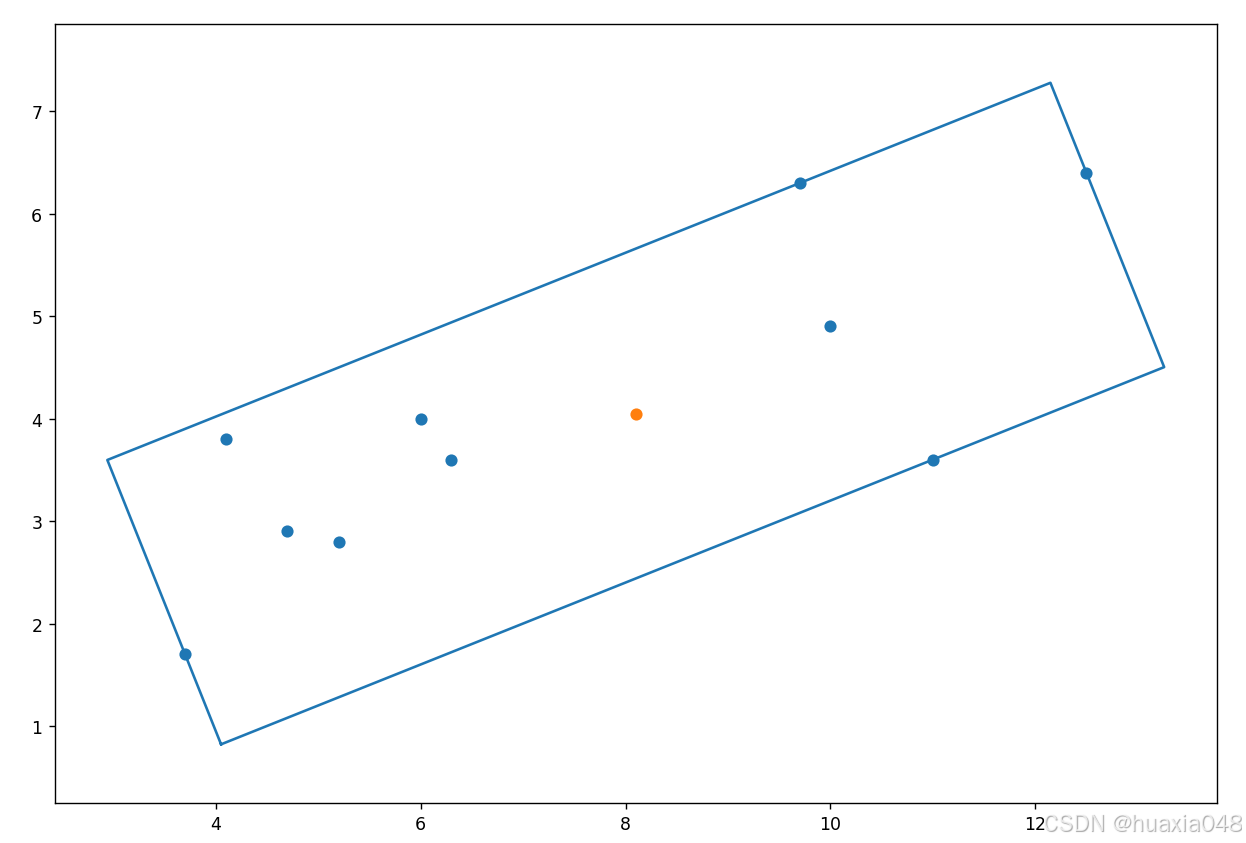
a  = np.array([(3.7, 1.7), (4.1, 3.8), (4.7, 2.9), (5.2, 2.8), (6.0,4.0), (6.3, 3.6), (9.7, 6.3), (10.0, 4.9), (11.0, 3.6), (12.5, 6.4)])
ca = np.cov(a,y = None,rowvar = 0,bias = 1)

v, vect = np.linalg.eig(ca)
tvect = np.transpose(vect)



fig = plt.figure(figsize=(12,12))
ax = fig.add_subplot(111)
ax.scatter(a[:,0],a[:,1])

#use the inverse of the eigenvectors as a rotation matrix and
#rotate the points so they align with the x and y axes
ar = np.dot(a,np.linalg.inv(tvect))

# get the minimum and maximum x and y
mina = np.min(ar,axis=0)
maxa = np.max(ar,axis=0)
diff = (maxa - mina)*0.5

# the center is just half way between the min and max xy
center = mina + diff

#get the 4 corners by subtracting and adding half the bounding boxes height and width to the center
corners = np.array([center+[-diff[0],-diff[1]],center+[diff[0],-diff[1]],center+[diff[0],diff[1]],center+[-diff[0],diff[1]],center+[-diff[0],-diff[1]]])

#use the the eigenvectors as a rotation matrix and
#rotate the corners and the centerback
corners = np.dot(corners,tvect)
center = np.dot(center,tvect)

ax.scatter([center[0]],[center[1]])
ax.plot(corners[:,0],corners[:,1],'-')

plt.axis('equal')
plt.show()

运行上述代码，