


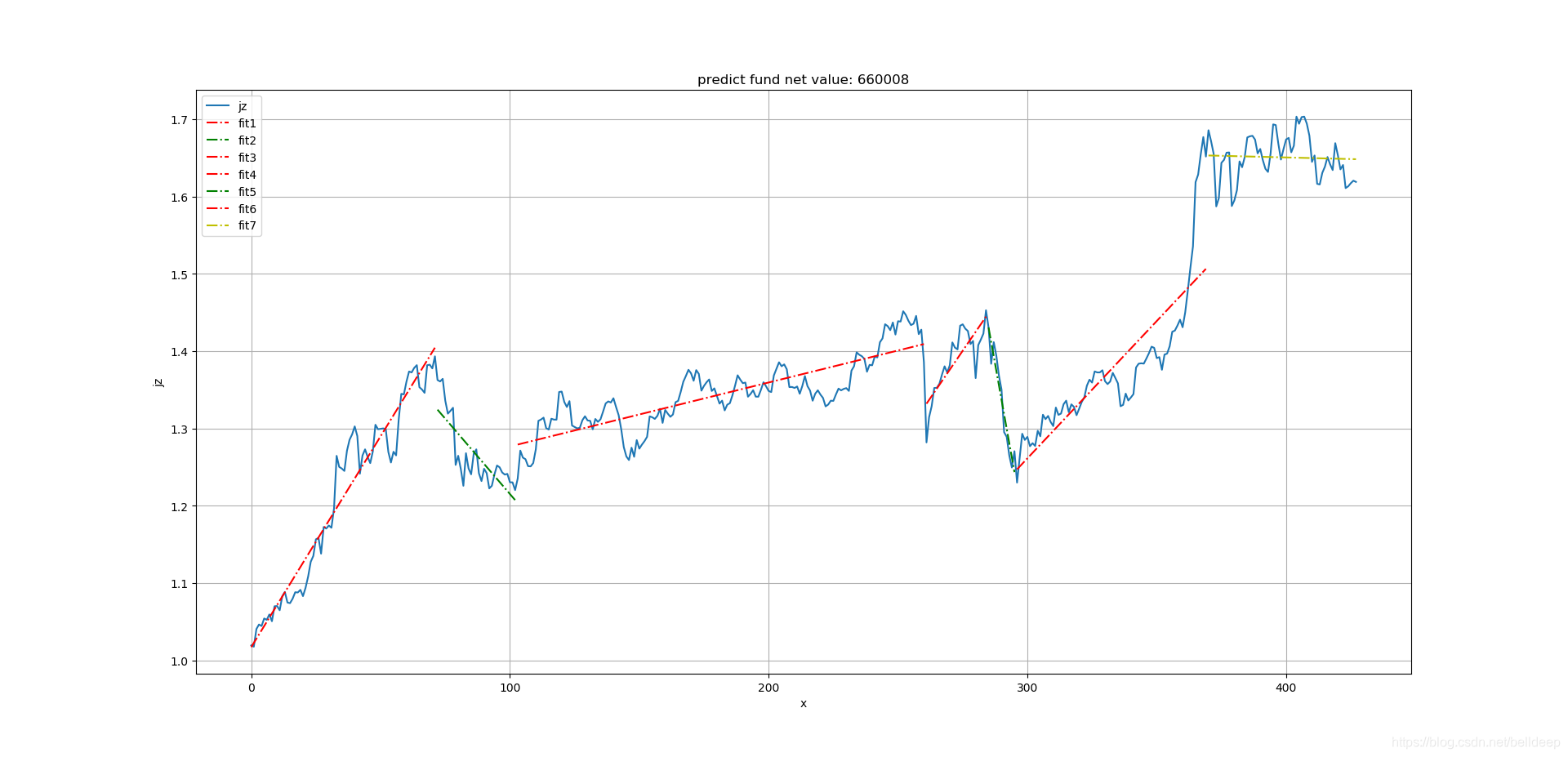
 本文通过一元线性回归分析了沪深300指数基金的净值变化趋势,并将其划分为七个时间段进行详细分析,同时展示了如何使用Python进行实际操作。
一元线性回归分析实例:时间序列分段
以沪深300指数基金净值为例
基金净值数据格式:date,jz,ljjz
2019-01-02,1.0194,1.0194
2019-01-03,1.0177,1.0177
linear_mod_2.py
# coding=utf-8
import os, sys
import numpy as np
import matplotlib.pyplot as plt
import pandas as pd
from sklearn.linear_model import LinearRegression
# python一元线性回归分析实例:指数基金净值
if len(sys.argv) ==2:
fcode = sys.argv[1]
else:
print('usage: python linear_mod_2.py fcode ')
sys.exit(1)
if len(fcode) !=6:
print(' fcode is char(6)')
sys.exit(2)
file1 = "./" +fcode +'.csv'
if not os.path.exists(file1):
print(file1 +' is not exists.')
sys.exit(3)
# 用pandas读取csv
df = pd.read_csv(file1)
df = df[ df['date'] > '2019-01-01']
df.index = pd.to_datetime(df.date)
y = df['jz'].values # 基金净值
x = np.arange(0,len(y),1)
# 构造X列表和Y列表,reshape(-1,1)改变数组形状,为只有一个属性
x = x.reshape(-1,1)
y = y.reshape(-1,1)
# 时间序列分段1
df1 = df[ df['date'] < '2019-04-20']
y1 = df1['jz'].values # 基金净值
x1 = np.arange(0,len(y1),1)
x1 = x1.reshape(-1,1)
y1 = y1.reshape(-1,1)
begin = len(y1)
# 时间序列分段2
dates = pd.date_range('2019-04-20','2019-06-09')
df2 = df[ df.index.isin(dates.values)]
y2 = df2['jz'].values # 基金净值
x2 = np.arange(begin, begin+len(y2),1)
x2 = x2.reshape(-1,1)
y2 = y2.reshape(-1,1)
begin = begin+len(y2)
# 时间序列分段3
dates = pd.date_range('2019-06-10','2020-01-24')
df3 = df[ df.index.isin(dates.values)]
y3 = df3['jz'].values # 基金净值
x3 = np.arange(begin, begin+len(y3),1)
x3 = x3.reshape(-1,1)
y3 = y3.reshape(-1,1)
begin = begin+len(y3)
# 时间序列分段4
dates = pd.date_range('2020-02-03','2020-03-05')
df4 = df[ df.index.isin(dates.values)]
y4 = df4['jz'].values # 基金净值
x4 = np.arange(begin, begin+len(y4),1)
x4 = x4.reshape(-1,1)
y4 = y4.reshape(-1,1)
begin = begin+len(y4)
# 时间序列分段5
dates = pd.date_range('2020-03-06','2020-03-20')
df5 = df[ df.index.isin(dates.values)]
y5 = df5['jz'].values # 基金净值
x5 = np.arange(begin, begin+len(y5),1)
x5 = x5.reshape(-1,1)
y5 = y5.reshape(-1,1)
begin = begin+len(y5)
# 时间序列分段6
dates = pd.date_range('2020-03-21','2020-07-11')
df6 = df[ df.index.isin(dates.values)]
y6 = df6['jz'].values # 基金净值
x6 = np.arange(begin, begin+len(y6),1)
x6 = x6.reshape(-1,1)
y6 = y6.reshape(-1,1)
begin = begin+len(y6)
# 时间序列分段7
df7 = df[ df['date'] > '2020-07-11']
y7 = df7['jz'].values # 基金净值
x7 = np.arange(begin, begin+len(y7),1)
x7 = x7.reshape(-1,1)
y7 = y7.reshape(-1,1)
begin = begin+len(y7)
# 构造回归对象
model = LinearRegression()
model.fit(x1, y1)
Y1 = model.predict(x1) # 获取预测值
model.fit(x2, y2)
Y2 = model.predict(x2)
model.fit(x3, y3)
Y3 = model.predict(x3)
model.fit(x4, y4)
Y4 = model.predict(x4)
model.fit(x5, y5)
Y5 = model.predict(x5)
model.fit(x6, y6)
Y6 = model.predict(x6)
model.fit(x7, y7)
Y7 = model.predict(x7)
# 构造返回字典
predictions = {}
predictions['intercept'] = model.intercept_ # 截距值
predictions['coefficient'] = model.coef_ # 回归系数(斜率值)
#predictions['predict_value'] = Y7
print(predictions)
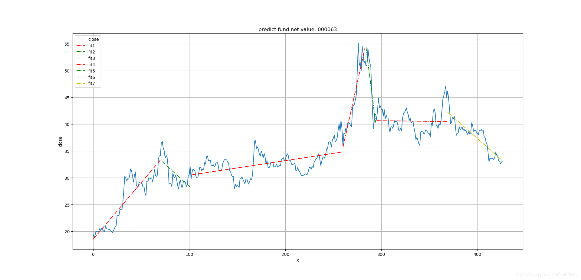
# 绘图
fig, ax = plt.subplots(figsize=(10,6))
# 绘出已知数据散点图
#plt.scatter(x, y, color ='blue')
# 绘曲线图
ax.plot(x, y, '-', label='jz') # 基金净值
# 绘出预测直线
ax.plot(x1, Y1, 'r--.', label='fit1')
ax.plot(x2, Y2, 'g--.', label='fit2')
ax.plot(x3, Y3, 'r--.', label='fit3')
ax.plot(x4, Y4, 'r--.', label='fit4')
ax.plot(x5, Y5, 'g--.', label='fit5')
ax.plot(x6, Y6, 'r--.', label='fit6')
ax.plot(x7, Y7, 'y--.', label='fit7')
ax.legend(loc='upper left')
plt.title('predict fund net value: ' +fcode)
plt.xlabel('x')
plt.ylabel('jz')
plt.grid()
plt.show()以沪深300指数基金净值为例
运行 python linear_mod_2.py 660008
以股票 000063 中兴通讯为例
运行 python stock1.py 000063
将 'jz' 全替换为 'close' 就可以为股票收盘价 做一元线性回归分析
运行 python linear_mod_2.py 000063


 1905
1905

 被折叠的 条评论
为什么被折叠?
被折叠的 条评论
为什么被折叠?
 到【灌水乐园】发言


