利用基于先验算法（PICCS）的fMRI研究的压缩传感重建中的时间冗余（Matlab代码实现）

 💥💥💞💞欢迎来到本博客❤️❤️💥💥

🏆博主优势：🌞🌞🌞博客内容尽量做到思维缜密，逻辑清晰，为了方便读者。

⛳️座右铭：行百里者，半于九十。

📋📋📋本文目录如下：🎁🎁🎁

目录

💥1 概述

目的：

方法：

结果：

结论：

📚2 运行结果

🎉3 参考文献

🌈4 Matlab代码实现

---

💥1 概述

文献来源：

目的：

压缩传感是一种用于在不影响图像质量的情况下加速磁共振成像 （MRI） 采集的技术。虽然它已被证明在心脏电影等动态成像程序中特别有用，但很少有作者将其应用于功能性磁共振成像 （fMRI）。本研究的目的是检查基于现有先验图像的先验图像约束压缩感知（PICCS）算法是否能够比其他利用时间冗余的策略更好地改善fMRI中的统计图。

方法：

PICCS 与时空总变异 （TTV） 和 k-t FASTER 进行了比较，因为它们已经在其他 MRI 应用中分别表现出高性能和稳健性，例如心脏电影 MRI 和静息态 fMRI。PICCS的先前图像是所有欠采样数据的平均值。PICCS和TTV均使用拆分Bregman公式求解。K-t FASTER算法依靠矩阵补全来重构欠采样的k空间。使用两个具有高信噪比和低信噪比 （SNR） 的数据集（BOLD 对比度）评估了这三种算法，这些数据集是在 7 T 临床前 MRI 扫描仪中采集的，并以不同的速率（即加速因子）进行回顾性欠采样。作者通过受试者工作特征曲线和统计图的目视检查，评估了BOLD检测的灵敏度/特异性。

结果：

在高信噪比研究中，PICCS的性能与最先进的算法TTV和k-t FASTER相似，并在ROI时提供一致的BOLD信号。在低信噪比和高加速因子的场景中，PICCS仍然提供一致的图谱和比TTV更高的灵敏度/特异性，而k-t FASTER未能提供显著的图谱。

结论：

作者对利用fMRI中时间冗余的三种重建（PICCS、TTV和k-t FASTER）进行了比较。在嘈杂场景中，基于先验的算法 PICCS 比 TTV 和 k-t FASTER 更好地保留了 BOLD 激活和灵敏度/特异性。PICCS 算法可能达到 ×8 的加速因子，并且仍然在 ROI 中提供粗体对比度，曲线下面积超过 0.99。

📚2 运行结果

 部分代码：

% Simulate data
data0       =   fft2(image0);         

%==========================================================================
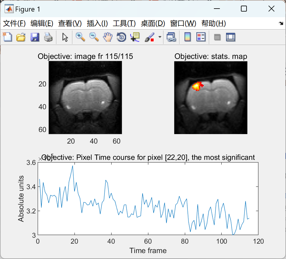
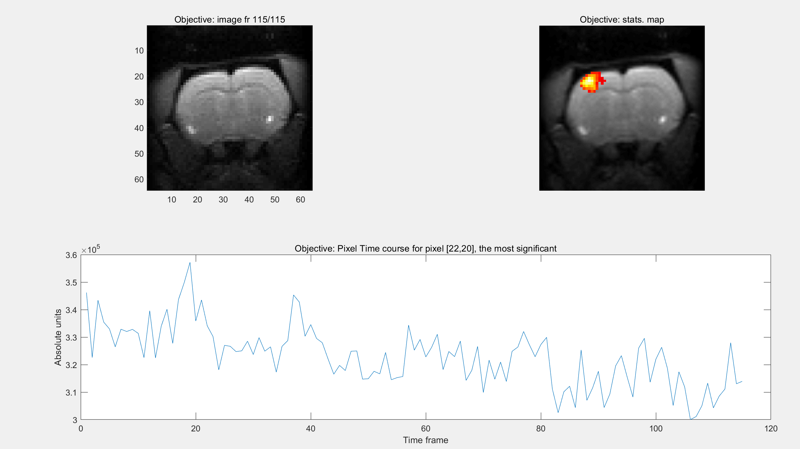
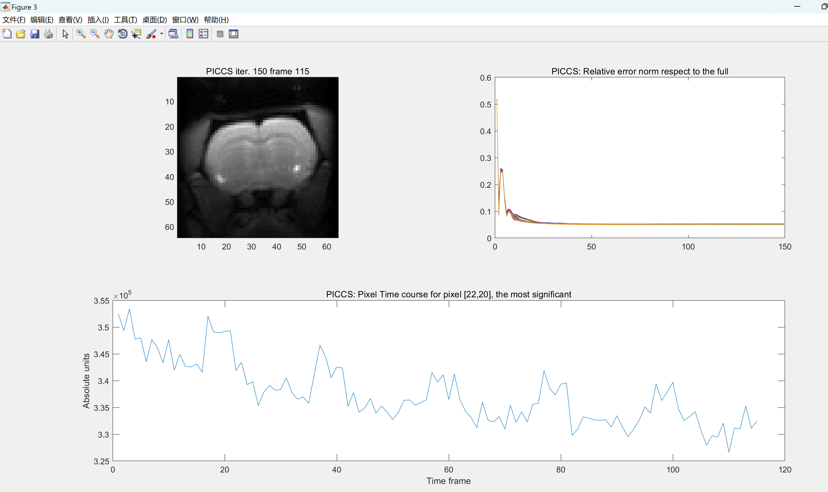
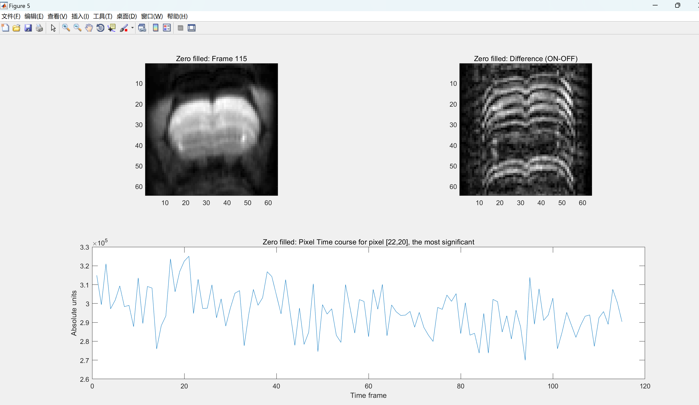
% DISPLAY FULL DATASET, highest activation pixel is [22,20]
%==========================================================================
% Here we display the thresholded statistical map obtained from the 
% original fully sampled dataset analyzed with: https://github.com/HGGM-LIM/fmrat
% As well as the fully sampled 115 frames in the simulated fMRI series and 
% the time course of the pixel [22,20], which yielded the highest statistical 
% t value.

% Display the statistical map
    close('all');
    scrs    =   get(0,'ScreenSize');
    h1       =   figure; set(h1,'Position',[30,scrs(4)/2,scrs(3)/3,scrs(4)*0.8/2]);
    subplot(2,2,2); imshow('map_full_p_0_01_k_12.tif'); title('Objective: stats. map');

% Display the time frames    
    subplot(2,2,1); 
    for i=1:115 
        figure(h1);
        imagesc(abs(image0(:,:,i))); title(['Objective: image fr ' num2str(i) '/115']); 
        colormap gray; axis image; drawnow;
        pause(0.05);
    end
    
% Display the time course of the highest activation pixel    
    tcourse=subplot(2,2,3:4);  plot(squeeze(image0(22,20,:))); title(tcourse,'Objective: Pixel Time course for pixel [22,20], the most significant')
    ylabel(tcourse,'Absolute units'),xlabel(tcourse,'Time frame');

    
%==========================================================================
% UNDERSAMPLE DATASET, choose an undersampling rate (1/acc. factor)
%==========================================================================
%     sp                   = [ ...
%                         0.05;...      % 5% of lines   
%                         0.1; ...      % 10% of lines 
%                         0.125;...     % 12.5% of lines 
%                         0.15;...      % 15% of lines   
%                         0.175;...     % 17.5% of lines 
%                         0.2; ...      % 20% of lines 
%                         0.3; ...      % 30% of lines 
%                         0.4; ...      % 40% of lines 
%                         0.5; ...      % 50% of lines 
%                         0.6; ...      % 60% of lines 
%                         0.7; ...      % 70% of lines 
%                         0.8; ...      % 80% of lines 
%                         0.9 ...       % 90% of lines 
%                             ];
%    The following are parameters required to generate the pdf at these
%    undersampling rates above:
%     Ps          =   [17,10,8,8,7.5,5,3,2,2,2,2,2,2];        % Decay
%     N           =   size(image0,1);                         % #phase enc lines
%     radius      =   [2/N ,3/N, 3.3/N, 3.7/N, 4.1/N, ...     % Central radius
%                     4.5/N,7/N,7/N,7/N,7/N,7/N,7/N,7/N];
        
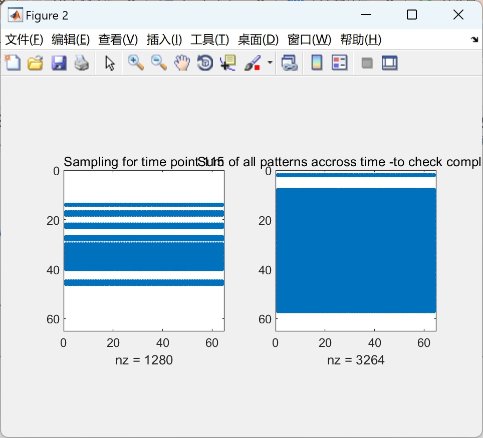
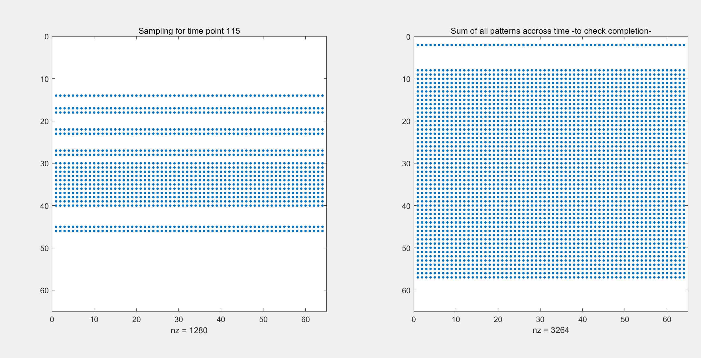
% To display the generated patterns for the 115 time frames
    h2          =   figure;
    set(h2,'Position',[30+scrs(3)/3,scrs(4)/2,scrs(3)/3,scrs(4)/2*0.8]);
    rname       =   'central_dense';
    
% Choose an undersampling rate (acc. factor)
    sp          =   0.3;     
    Ps          =   3;
    radius      =   7/size(image0,1);
    
% Create an undersampling for each time frame and display them
    dims        =   size(image0);
    RAll        =   genRAll(dims,sp,Ps,radius,pwd,rname,h2);
    fprintf('Generated RAll %s\t for sparsity: %s \r\n',rname, num2str(sp));                    

% Display the sum of the undersamplings along time to check the kspace completion 
    RAll_visu   =   fftshift(RAll);
    figure(h2),subplot(1,2,2),
    spy(squeeze(sum(RAll_visu,3))), 100*nnz(squeeze(sum(RAll_visu,3)))/size(image0,1)
    title('Sum of all patterns accross time -to check completion-');

🎉3 参考文献

文章中一些内容引自网络，会注明出处或引用为参考文献，难免有未尽之处，如有不妥，请随时联系删除。

🌈4 Matlab代码实现