脱发因素可视化分析及机器学习预测

资料来源
该数据集记录了可能导致个体脱发的各种因素，每行代表一位独特的个体，列则涵盖了遗传、荷尔蒙变化、医疗状况、药物和治疗、营养缺乏、压力水平、年龄、不良护发习惯、环境因素、吸烟习惯、体重减轻以及脱发的有无等信息。

1. 数据可视化分析

import pandas as pd
import matplotlib.pyplot as plt
import seaborn as sns
import numpy as np
from sklearn.model_selection import train_test_split
from sklearn.ensemble import RandomForestClassifier
from sklearn.preprocessing import LabelEncoder
from sklearn.metrics import classification_report, roc_curve, auc, confusion_matrix
import xgboost as xgb
from sklearn.svm import SVC
import warnings
warnings.filterwarnings('ignore')

1.1 数据预处理

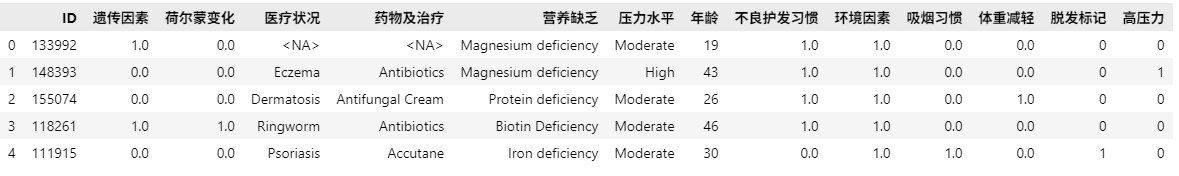
# 数据预处理
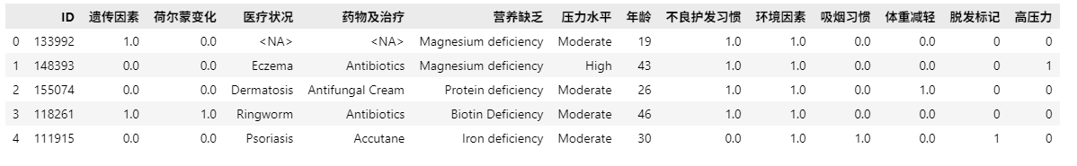
df = pd.read_csv("/home/mw/input/data5086/archive/Predict Hair Fall.csv")
df.head(5)

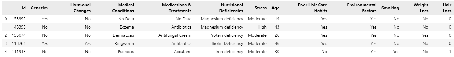
怕代码不显示，故插入图片

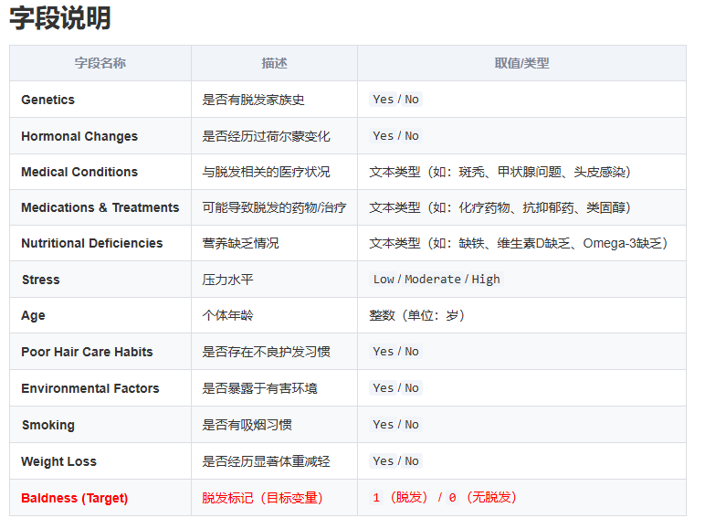
字段说明

字段名称	描述	取值/类型
Genetics	是否有脱发家族史	Yes/No
Hormonal Changes	是否经历过荷尔蒙变化	Yes/No
Medical Conditions	与脱发相关的医疗状况	文本类型（如：斑秃、甲状腺问题、头皮感染）
Medications & Treatments	可能导致脱发的药物/治疗	文本类型（如：化疗药物、抗抑郁药、类固醇）
Nutritional Deficiencies	营养缺乏情况	文本类型（如：缺铁、维生素D缺乏、Omega-3缺乏）
Stress	压力水平	Low/Moderate/High
Age	个体年龄	整数（单位：岁）
Poor Hair Care Habits	是否存在不良护发习惯	Yes/No
Environmental Factors	是否暴露于有害环境	Yes/No
Smoking	是否有吸烟习惯	Yes/No
Weight Loss	是否经历显著体重减轻	Yes/No
Baldness (Target)	脱发标记（目标变量）	1（脱发） / 0（无脱发）

1.2 标准化列名

部分英文列名可能会不标准或者乱码，所以自己定义一下

# 定义中文列名（12个特征和目标）
chinese_columns = [
    '遗传因素', 
    '荷尔蒙变化', 
    '医疗状况', 
    '药物及治疗', 
    '营养缺乏', 
    '压力水平', 
    '年龄', 
    '不良护发习惯', 
    '环境因素', 
    '吸烟习惯', 
    '体重减轻', 
    '脱发标记'   # 目标变量
]

# 将原始数据集的列名改为：第一列为'ID'，后面依次为chinese_columns中的12个列名
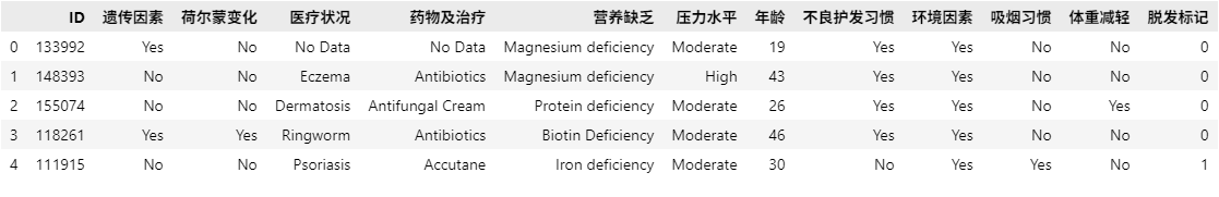
df.columns = ['ID'] + chinese_columns
df.head(5)

1.3 缺失值处理

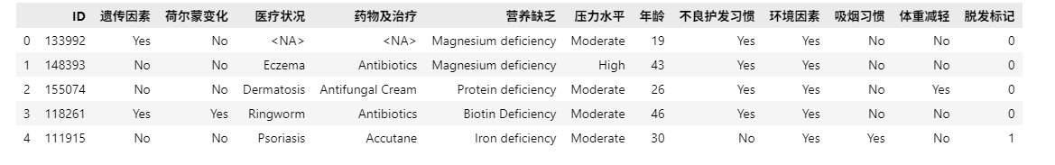
# 缺失值处理
df.replace("No Data", pd.NA, inplace=True)
df.head(5)

1.4 部分字段处理

# 二值列转换
binary_cols = ['遗传因素', '荷尔蒙变化', '不良护发习惯', '环境因素', '吸烟习惯', '体重减轻']
for col in binary_cols:
    df[col] = df[col].map({'Yes': 1, 'No': 0, pd.NA: np.nan})

# 创建高压力分组
df['高压力'] = df['压力水平'].apply(lambda x: 1 if x == 'High' else 0)
df.head(5)

df.head(5)

1.5 数据可视化

脱发标记分布

# 脱发标记分布
plt.figure(figsize=(8, 5))
sns.countplot(x='脱发标记', data=df, legend=False, hue='脱发标记',  palette=['#7fcdbb', '#2c7fb8'])
plt.title('脱发标记分布 (0=无脱发, 1=有脱发)', fontsize=14)
plt.xlabel('')
plt.ylabel('样本数量', fontsize=12)
plt.xticks([0, 1], ['无脱发', '有脱发'], fontsize=12)
plt.tight_layout()
plt.show()

# 计算脱发比例
hair_loss_rate = df['脱发标记'].mean() * 100
print(f"脱发比例: {hair_loss_rate:.1f}%")

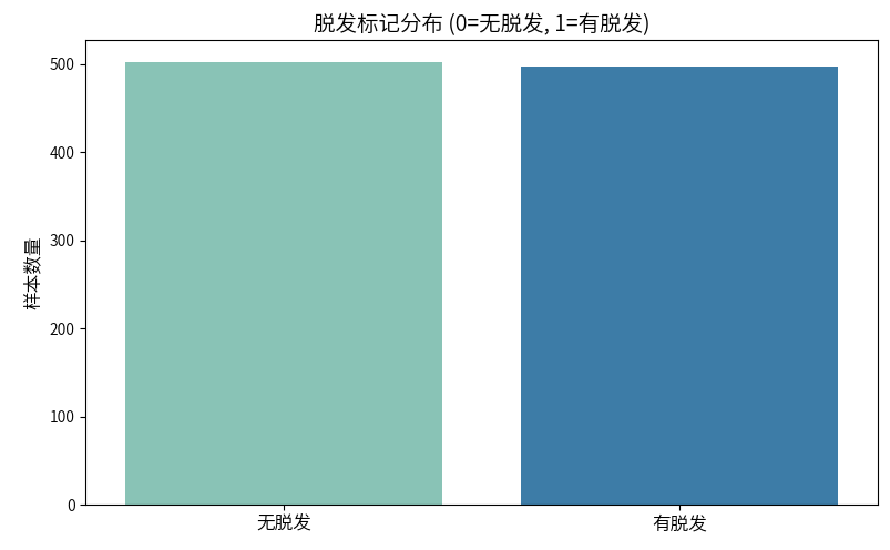
脱发比例: 49.7%

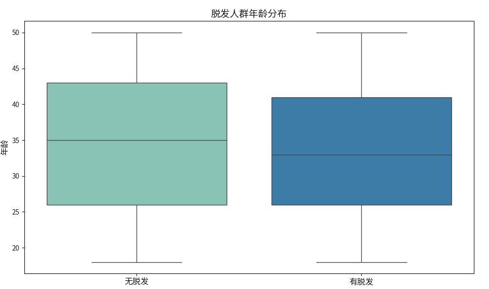
年龄与脱发关系

# 年龄与脱发关系
plt.figure(figsize=(10, 6))
sns.boxplot(x='脱发标记', y='年龄', data=df, legend=False, hue='脱发标记', palette=['#7fcdbb', '#2c7fb8'])
plt.title('脱发人群年龄分布', fontsize=14)
plt.xlabel('')
plt.ylabel('年龄', fontsize=12)
plt.xticks([0, 1], ['无脱发', '有脱发'], fontsize=12)
plt.tight_layout()
plt.show()

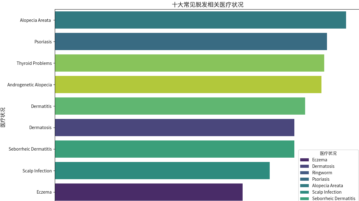
常见医疗状况分析

# 常见医疗状况分析
plt.figure(figsize=(12, 8))
top_conditions = df['医疗状况'].value_counts().head(10).index
ax = sns.countplot(y='医疗状况', data=df, hue = '医疗状况',
               order=top_conditions, 
               palette=sns.color_palette("viridis", 10))

plt.title('十大常见脱发相关医疗状况', fontsize=14)
plt.xlabel('样本数量', fontsize=12)
plt.ylabel('医疗状况', fontsize=12)
plt.tight_layout()
plt.show()

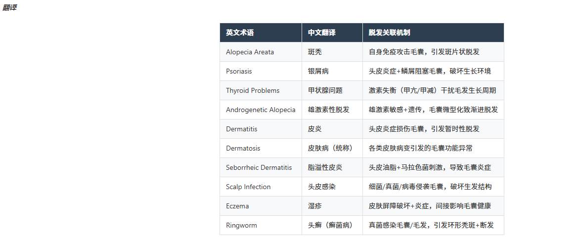
翻译

英文术语	中文翻译	脱发关联机制
Alopecia Areata	斑秃	自身免疫攻击毛囊，引发斑片状脱发
Psoriasis	银屑病	头皮炎症+鳞屑阻塞毛囊，破坏生长环境
Thyroid Problems	甲状腺问题	激素失衡（甲亢/甲减）干扰毛发生长周期
Androgenetic Alopecia	雄激素性脱发	雄激素敏感+遗传，毛囊微型化致渐进脱发
Dermatitis	皮炎	头皮炎症损伤毛囊，引发暂时性脱发
Dermatosis	皮肤病（统称）	各类皮肤病变引发的毛囊功能异常
Seborrheic Dermatitis	脂溢性皮炎	头皮油脂+马拉色菌刺激，导致毛囊炎症
Scalp Infection	头皮感染	细菌/真菌/病毒侵袭毛囊，破坏生发结构
Eczema	湿疹	皮肤屏障破坏+炎症，间接影响毛囊健康
Ringworm	头癣（癣菌病）	真菌感染毛囊/毛发，引发环形秃斑+断发

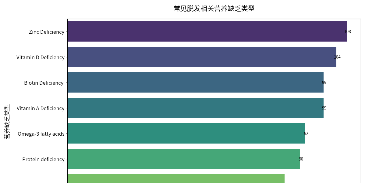
常见脱发相关营养缺乏类型

plt.figure(figsize=(12, 8))

# 获取Top8类别
top_nutrition = df['营养缺乏'].value_counts().head(8).index

ax = sns.countplot(
    y='营养缺乏',
    data=df,
    hue='营养缺乏',
    order=top_nutrition,        
    hue_order=top_nutrition,    
    palette=sns.color_palette("viridis", len(top_nutrition)),  # 动态匹配颜色数量
    legend=False
)

# 添加数据标签
for p in ax.patches:
    ax.annotate(f'{int(p.get_width())}', 
                (p.get_width() + 0.3, p.get_y() + p.get_height()/2),
                ha='center', va='center', fontsize=10)

plt.title('常见脱发相关营养缺乏类型', fontsize=16, pad=20)
plt.xlabel('样本数量', fontsize=14)
plt.ylabel('营养缺乏类型', fontsize=14)
plt.xticks(fontsize=12)
plt.yticks(fontsize=12)

plt.tight_layout()
plt.show()

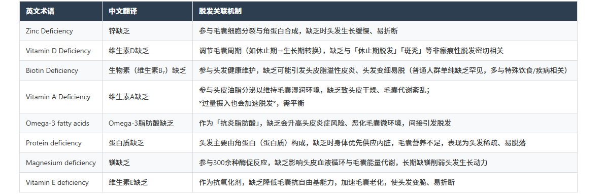
英文术语	中文翻译	脱发关联机制
Zinc Deficiency	锌缺乏	参与毛囊细胞分裂与角蛋白合成，缺乏时头发生长缓慢、易折断
Vitamin D Deficiency	维生素D缺乏	调节毛囊周期（如休止期→生长期转换），缺乏与「休止期脱发」「斑秃」等非瘢痕性脱发密切相关
Biotin Deficiency	生物素（维生素B₇）缺乏	参与头发健康维护，缺乏可能引发头皮脂溢性皮炎、头发变细易脱（普通人群单纯缺乏罕见，多与特殊饮食/疾病相关）
Vitamin A Deficiency	维生素A缺乏	参与头皮油脂分泌以维持毛囊湿润环境，缺乏致头皮干燥、毛囊代谢紊乱； *过量摄入也会加速脱发*，需平衡
Omega-3 fatty acids	Omega-3脂肪酸缺乏	作为「抗炎脂肪酸」，缺乏会升高头皮炎症风险、恶化毛囊微环境，间接引发脱发
Protein deficiency	蛋白质缺乏	头发主要由角蛋白（蛋白质）构成，缺乏时身体优先供应内脏，毛囊营养不足，表现为头发稀疏、易脱落
Magnesium deficiency	镁缺乏	参与300余种酶促反应，缺乏影响头皮血液循环与毛囊能量代谢，长期缺镁削弱头发生长动力
Vitamin E deficiency	维生素E缺乏	作为抗氧化剂，缺乏降低毛囊抗自由基能力，加速毛囊老化，使头发变脆、易折断

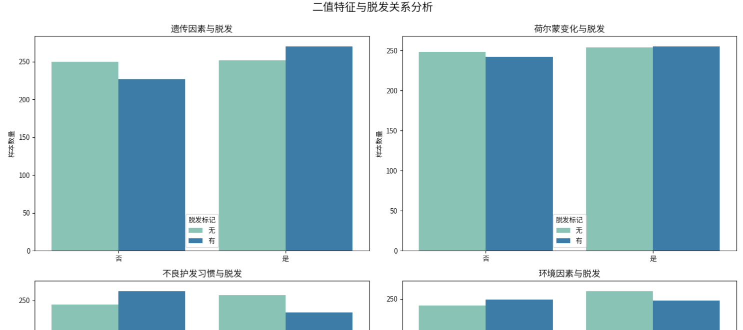
二值特征与脱发关系

# 二值特征与脱发关系
features = ['遗传因素', '荷尔蒙变化', '不良护发习惯', '环境因素', '吸烟习惯', '体重减轻']

fig, axes = plt.subplots(3, 2, figsize=(15, 15))
axes = axes.flatten()

for i, feature in enumerate(features):
    if i < len(axes):
        sns.countplot(x=feature, hue='脱发标记', data=df, 
                     palette=['#7fcdbb', '#2c7fb8'], ax=axes[i])
        axes[i].set_title(f'{feature}与脱发', fontsize=13)
        axes[i].set_xlabel('')
        axes[i].set_xticklabels(['否' if t == 0 else '是' for t in [0, 1]])
        axes[i].set_ylabel('样本数量')
        axes[i].legend(title='脱发标记', labels=['无', '有'])

plt.tight_layout()
plt.suptitle('二值特征与脱发关系分析', fontsize=16, y=1.02)
plt.show()

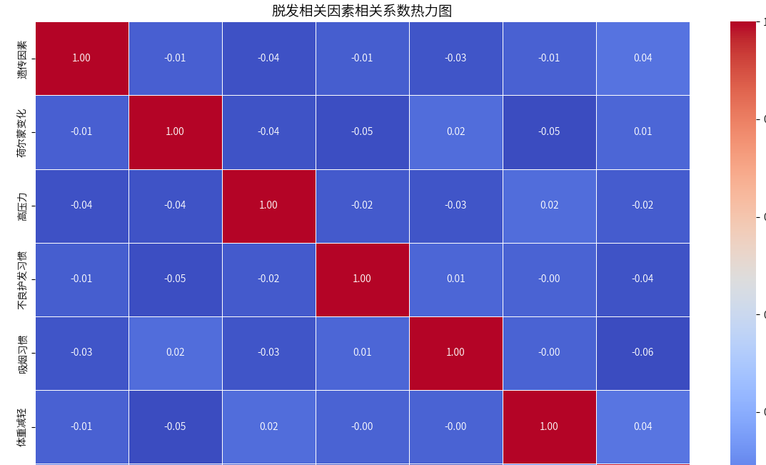
特征相关性分析

# 特征相关性分析
corr_features = ['遗传因素', '荷尔蒙变化', '高压力', '不良护发习惯', '吸烟习惯', '体重减轻', '脱发标记']
corr = df[corr_features].corr()
plt.figure(figsize=(12, 8))
sns.heatmap(corr, annot=True, cmap='coolwarm', fmt=".2f", linewidths=.5)
plt.title('脱发相关因素相关系数热力图', fontsize=14)
plt.tight_layout()
plt.show()

2. 模型预测

使用随机森林及xgboost

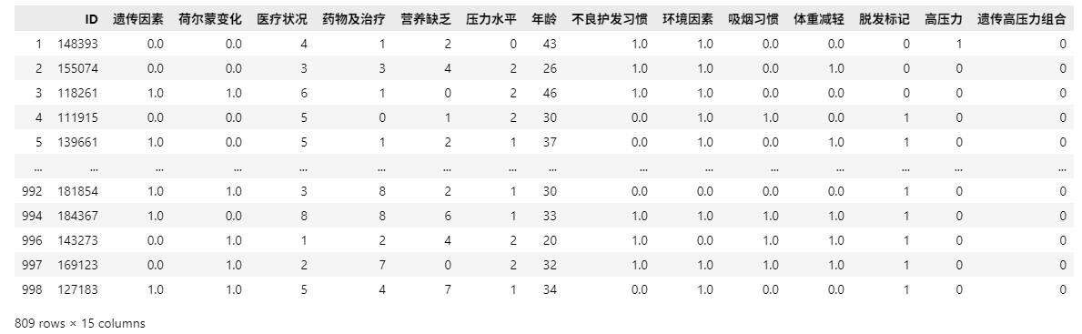
df.head(5)

2.1 特征工程

字段处理及编码

# 缺失值处理（删除少量缺失行）
df.dropna(subset=['脱发标记', '医疗状况', '药物及治疗', '营养缺乏'], inplace=True)
# 复合变量
# 遗传因素+高压力组合
df['遗传高压力组合'] = ((df['遗传因素'] == 1) & (df['高压力'] == 1)).astype(int)

# 标签编码分类变量
label_encoders = {}
categorical_cols = ['医疗状况', '药物及治疗', '营养缺乏', '压力水平']
for col in categorical_cols:
    le = LabelEncoder()
    df[col] = le.fit_transform(df[col].astype(str))
    label_encoders[col] = le

2.2 数据集划分

数据集比例选择85：15，因为数据太少了

# 特征选择（部分可能部分重复，但影响不大）
features = [
    '遗传因素', '荷尔蒙变化', '医疗状况', '药物及治疗', 
    '营养缺乏', '压力水平', '年龄', '不良护发习惯', 
    '环境因素', '吸烟习惯', '体重减轻', '高压力',
    '遗传高压力组合'
]

X = df[features]
y = df['脱发标记']

# 划分训练集和测试集
X_train, X_test, y_train, y_test = train_test_split(
    X, y, test_size=0.15, random_state=42, stratify=y
)

2.3 选择模型并自适应参数

from sklearn.model_selection import GridSearchCV

param_grid_rf = {
    'n_estimators': [50, 100],
    'max_depth': [5, 7],
    'min_samples_split': [10, 15],
    'class_weight': ['balanced', None]
}

grid_rf = GridSearchCV(
    RandomForestClassifier(random_state=42),
    param_grid_rf,
    cv=3,        # 小数据用3折交叉验证（减少计算量）
    scoring='f1',# 用F1平衡precision/recall
    n_jobs=-1    # 并行加速
)
grid_rf.fit(X_train, y_train)
best_rf = grid_rf.best_estimator_

param_grid_xgb = {
    'n_estimators': [50, 100],
    'max_depth': [3, 5],
    'learning_rate': [0.1, 0.2],
    'subsample': [0.8, 0.9],
    'colsample_bytree': [0.8, 0.9]
}

grid_xgb = GridSearchCV(
    xgb.XGBClassifier(objective='binary:logistic', random_state=42),
    param_grid_xgb,
    cv=3,
    scoring='f1',
    n_jobs=-1
)
grid_xgb.fit(X_train, y_train)
best_xgb = grid_xgb.best_estimator_

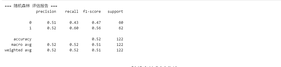
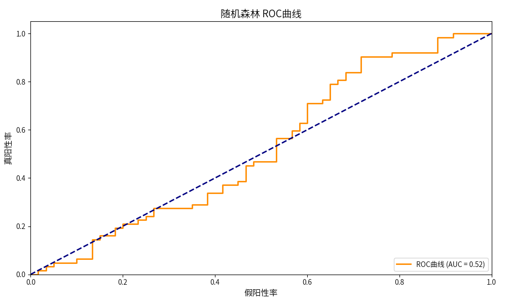
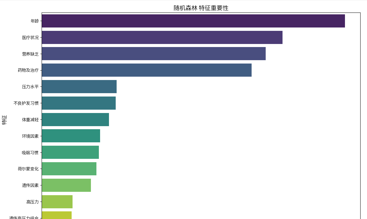
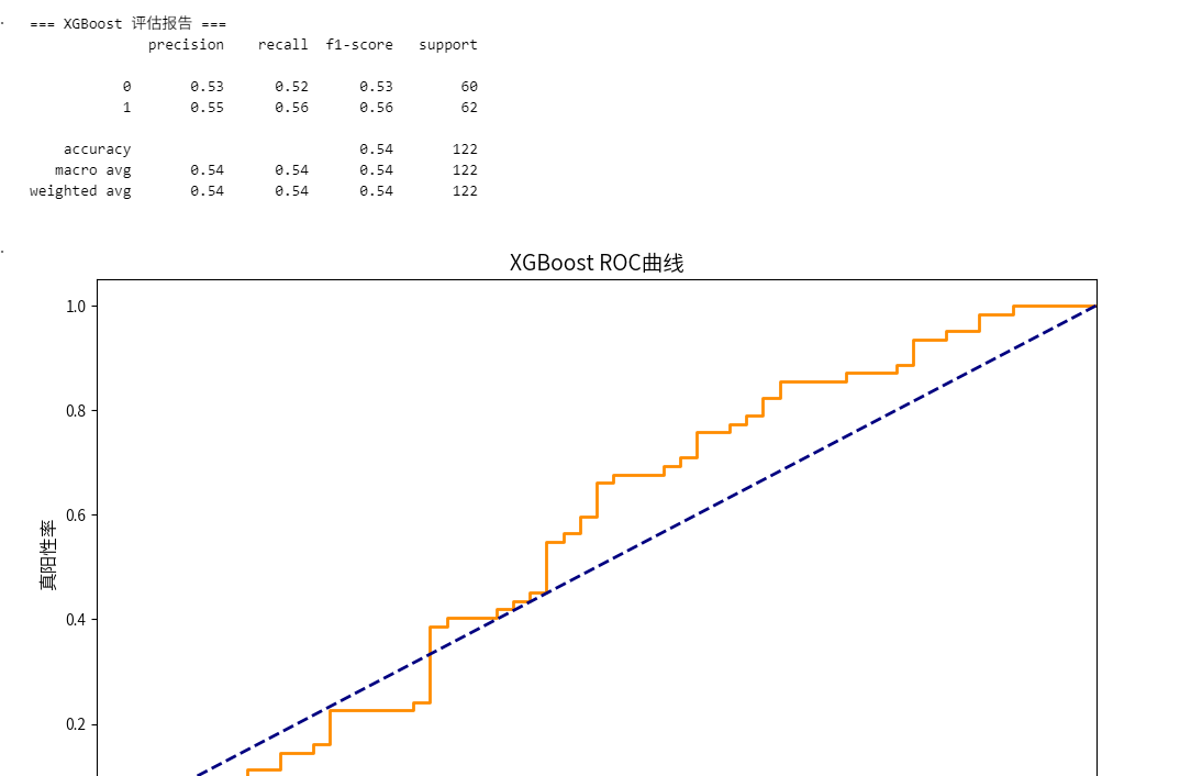
2.4 定义模型评估函数

# 模型评估函数
def evaluate_model(model, X_test, y_test, model_name):
    """评估模型并绘制ROC曲线"""
    y_pred = model.predict(X_test)
    y_proba = model.predict_proba(X_test)[:, 1]
    
    # 评估报告
    print(f"=== {model_name} 评估报告 ===")
    print(classification_report(y_test, y_pred))
    
    # ROC曲线
    fpr, tpr, thresholds = roc_curve(y_test, y_proba)
    roc_auc = auc(fpr, tpr)
    
    plt.figure(figsize=(10, 6))
    plt.plot(fpr, tpr, color='darkorange', lw=2, 
             label=f'ROC曲线 (AUC = {roc_auc:.2f})')
    plt.plot([0, 1], [0, 1], color='navy', lw=2, linestyle='--')
    plt.xlim([0.0, 1.0])
    plt.ylim([0.0, 1.05])
    plt.xlabel('假阳性率', fontsize=12)
    plt.ylabel('真阳性率', fontsize=12)
    plt.title(f'{model_name} ROC曲线', fontsize=14)
    plt.legend(loc="lower right")
    plt.tight_layout()
    plt.show()
    
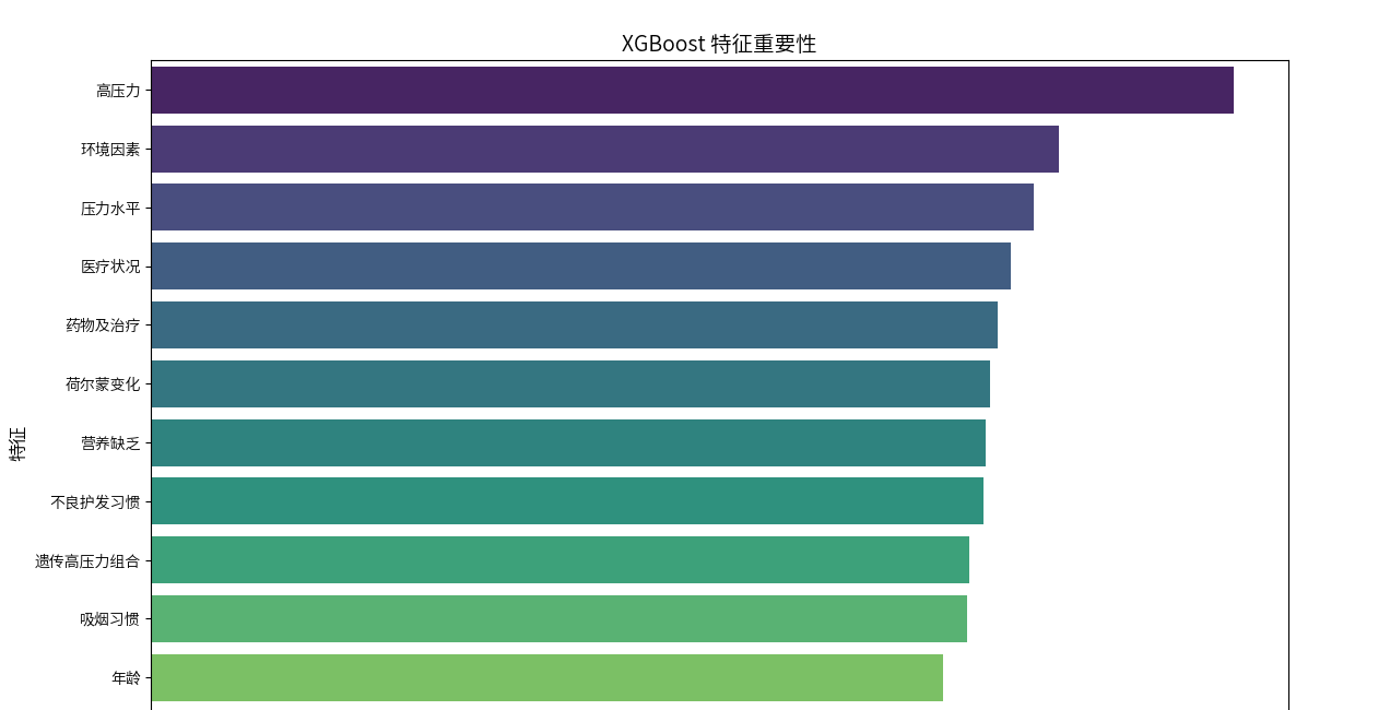
    # 特征重要性
    if hasattr(model, 'feature_importances_'):
        feature_imp = pd.DataFrame({
            '特征': features,
            '重要性': model.feature_importances_
        }).sort_values('重要性', ascending=False)
        
        plt.figure(figsize=(12, 8))
        sns.barplot(x='重要性', y='特征', data=feature_imp, palette='viridis')
        plt.title(f'{model_name} 特征重要性', fontsize=14)
        plt.xlabel('重要性', fontsize=12)
        plt.ylabel('特征', fontsize=12)
        plt.tight_layout()
        plt.show()
    
    return roc_auc

2.5 评估模型

由于数据很少，所以不是很准，但是模型训练步骤差不多就这样了
如果觉得准确率太低可以使用重采样或过采样生成点数据

# 评估模型
rf_auc = evaluate_model(best_rf, X_test, y_test, "随机森林")
xgb_auc = evaluate_model(best_xgb, X_test, y_test, "XGBoost")

资料来源