跨模态智能脑肿瘤检测

资料引用

跨模态智能脑肿瘤检测

基于多模态CT与MRI图像的深度学习优化模型

前言

脑肿瘤的早期检测和诊断对患者的治疗效果至关重要。随着医疗成像技术的进步，**计算机断层扫描（CT）和磁共振成像（MRI）**已成为最常用的脑部影像学检查方法。这些成像技术能够提供关于脑部结构和病变的关键信息，帮助医生准确地诊断肿瘤类型和位置。然而，传统的人工诊断依赖医生的经验，且常常受到主观因素的影响，特别是在复杂或早期的肿瘤案例中，准确性和效率可能受到限制。

因此，利用机器学习和深度学习技术对这些医学图像进行自动化分析，成为近年来医学影像领域的一个重要研究方向。通过使用计算机视觉和人工智能算法，能够有效地帮助医生提高诊断的准确率和效率，尤其是在资源有限的医疗环境中，这种技术能够提供快速、准确的辅助决策。

背景

在脑肿瘤的检测中，不同类型的成像技术（如CT和MRI）各有其优缺点。例如，CT扫描可以提供快速、详细的脑部骨骼结构信息，但对软组织的分辨率较低。而MRI扫描则能提供高分辨率的软组织图像，尤其对于脑肿瘤和其他软组织病变的识别尤为有效。

但是，单一模态的图像有时难以提供足够的全面信息。多模态影像融合，通过结合不同类型的成像技术（如CT与MRI），能够更全面地捕捉到肿瘤的各种特征，进而提高肿瘤检测的准确性。因此，使用多模态图像数据来训练深度学习模型，成为了提高脑肿瘤分类和检测精度的有效途径。

项目目的

本项目的目标是基于CT和MRI扫描的多模态数据，建立并优化一个深度学习模型，以准确地检测和分类脑肿瘤。具体任务包括：

• 处理和预处理CT与MRI图像数据。
• 利用卷积神经网络（CNN）或迁移学习模型（如EfficientNet）对脑肿瘤进行分类。
• 通过数据增强和类平衡策略，提高模型在实际应用中的鲁棒性。
• 评估并优化模型的性能，以确保其在临床环境中的有效性。

通过本项目，我们期望能够为医疗行业提供一个高效、可靠的自动化工具，辅助医生更早期、更准确地诊断脑肿瘤，进而改善患者的治疗效果和生存率。

实际应用

该模型可以广泛应用于以下领域：

1. 临床诊断辅助：提高脑肿瘤的诊断效率，特别是在资源有限或专家数量不足的地区，机器学习模型可以为医生提供有力的支持。
2. 肿瘤筛查：对于高风险人群，自动化的肿瘤筛查系统可以帮助早期发现潜在的脑部疾病，提高治疗的成功率。
3. 医疗影像分析自动化：随着医学影像数据量的不断增加，人工分析的负担越来越大。通过自动化的图像分析系统，可以减少医生的工作压力，提高医疗服务的效率。

通过本项目开发的模型，未来将为脑肿瘤的早期检测、定量分析和个性化治疗方案的制定提供宝贵的支持，推动医学人工智能的发展，为全球患者带来更好的医疗服务。

项目所使用的模型：EfficientNetB0

在这个脑肿瘤多模态图像（CT与MRI）分类项目中，核心的深度学习模型是 EfficientNetB0。EfficientNet 是 Google 在 2019 年提出的一种高效卷积神经网络架构，它在分类精度和计算效率之间取得了良好的平衡。EfficientNet 系列模型通过一种 复合缩放 方法，通过调整网络的宽度、深度和分辨率来最优化模型的性能。

本项目使用的 EfficientNetB0 是 EfficientNet 系列中的基础版本，尽管它较为轻量，但在许多计算机视觉任务中依然表现出色。

1. EfficientNetB0 概述

EfficientNetB0 是 EfficientNet 系列中的第一个模型，它采用了一种新的模型设计方法来提高网络的效率。与传统的网络（如ResNet、VGG等）不同，EfficientNet 通过复合缩放的方法，同时缩放网络的深度、宽度和分辨率，而不是单纯地增加某一维度。这样做能够在保持计算量相对较小的情况下，显著提升模型的性能。

EfficientNet 的核心创新点是 复合缩放（Compound Scaling）。传统的网络设计中，增加深度或宽度通常会增加计算量，但 EfficientNet 提出了通过同时增加深度、宽度和分辨率来优化网络性能，而不是单独优化某一个维度。

**EfficientNet 的复合缩放策略： **

• 深度（Depth）：增加网络的层数，能够让模型学习更复杂的特征。
• 宽度（Width）：增加每层的神经元数量，能够让每层捕获更多的特征。
• 分辨率（Resolution）：增大输入图像的分辨率，以便捕获更多的细节信息。

EfficientNet 的设计使得它在 参数量 和 计算量 之间取得了很好的平衡，从而在多个标准数据集上获得了优异的性能。

2. 为什么选择 EfficientNetB0

选择 EfficientNetB0 的原因主要包括以下几点：

• 预训练权重：EfficientNetB0 在大规模数据集（如 ImageNet）上进行了预训练，这使得它能够利用现有的知识来加速在特定任务上的训练，尤其适合迁移学习。

• 高效性：EfficientNetB0 是一个高效的网络，能够在较少的计算资源下实现较高的准确率。相比于传统的网络（如 ResNet 或 VGG），它能够在相同的计算量下达到更好的性能。

• 迁移学习：EfficientNetB0 在 ImageNet 数据集上进行了大规模预训练，因此能够很好地适应不同的计算机视觉任务。迁移学习可以有效地减少训练时间并提高性能。

• 小模型规模：EfficientNetB0 比其他更复杂的 EfficientNet 模型（如B1、B2等）小且快速，适合本项目中的资源限制，尤其是在图像预处理和训练阶段的效率方面表现出色。

3. EfficientNetB0 的架构

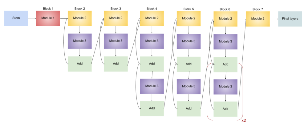
EfficientNetB0 的架构基于 Mobile Inverted Bottleneck Convolution（MBConv）模块，主要由以下部分组成：

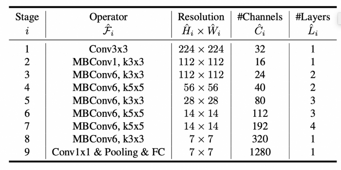
1. Stem Block：负责对输入图像进行初步处理，并提取特征。
2. MBConv Block：这是 EfficientNet 的核心部分，通过逐层增加通道数、宽度等来逐步提取更多特征。它利用深度可分离卷积来减少计算量。
3. Depthwise Separable Convolutions：这种卷积方式能够显著减少参数数量和计算量，是 EfficientNet 设计中的一个关键组件。
4. Global Average Pooling：该操作将每个特征图的空间维度平均化，以生成固定大小的输出。
5. 全连接层与输出层：在最后的全连接层后，采用 Softmax 或 Sigmoid 激活函数来进行分类任务的输出。

4. EfficientNetB0 在本项目中的应用

迁移学习
本项目使用了 迁移学习 技术，将预训练的 EfficientNetB0 模型应用到脑肿瘤分类任务中。具体做法是：

• 使用 EfficientNetB0 的预训练权重（来自 ImageNet 数据集），冻结网络的底层卷积层（即不对其进行训练）。
• 对网络的顶部进行微调：添加 全局平均池化（Global Average Pooling） 层，全连接层 和 Dropout 层，最终通过 Sigmoid 激活函数进行二分类（健康/肿瘤）。

通过冻结底层卷积层，本项目能够避免计算量过大，并利用预训练权重加速模型的训练过程。

模型输出层
最终的输出层是一个 Sigmoid 激活函数，用于处理二分类任务：

• 0（健康）：表示没有脑肿瘤的图像。
• 1（肿瘤）：表示图像中存在脑肿瘤。

模型的损失函数使用 binary_crossentropy，并通过 Adam 优化器进行优化。

5. EfficientNetB0 在训练中的表现

在本项目中，使用 EfficientNetB0 训练模型并进行 二分类任务，模型的评估结果表明它能够较好地学习到脑肿瘤与健康图像之间的差异。在训练过程中，通过数据增强、类平衡策略（使用 class_weight）等方法进一步提升了模型的鲁棒性。

通过适当的调优和回调机制（如早停、模型检查点保存等），模型能够快速收敛，避免过拟合，并且在验证集和测试集上表现出色。

!pip install opencv-python -i  https://mirrors.aliyun.com/pypi/simple/

import os, glob
import matplotlib.pyplot as plt
import seaborn as sns
import numpy as np
from tensorflow.keras.callbacks import EarlyStopping, ModelCheckpoint, ReduceLROnPlateau
from sklearn.utils import class_weight
from sklearn.model_selection import train_test_split
from tensorflow.keras.preprocessing.image import ImageDataGenerator
from tensorflow.keras.applications.efficientnet import preprocess_input
from tensorflow.keras.applications import EfficientNetB0
from tensorflow.keras.models import Model
from tensorflow.keras.layers import Dense, GlobalAveragePooling2D, Dropout
from tensorflow.keras.optimizers import Adam
from sklearn.metrics import classification_report, confusion_matrix, roc_curve, auc
import tensorflow as tf
import random
import pandas as pd
import cv2
sns.set()

1. 数据导入与预处理

1.1 数据加载与组织

数据集包括CT与MRI两种不同模态的图像数据，分别来自健康与肿瘤患者。代码通过使用Python的glob库读取图像文件，并将文件路径和标签（肿瘤/健康）存储在一个DataFrame中，方便后续操作。

#I imported it locally, however, It can be done with any method preferred. 
dataDirectory = "/home/mw/input/1111111111111113949/Brain tumor multimodal image/Dataset"

ctHealthyPath = glob.glob(os.path.join(dataDirectory, "Brain Tumor CT scan Images", "Healthy", "*.jpg"))
ctTumorPath  = glob.glob(os.path.join(dataDirectory, "Brain Tumor CT scan Images", "Tumor", "*.jpg"))

mriHealthyPath = glob.glob(os.path.join(dataDirectory, "Brain Tumor MRI images", "Healthy", "*.jpg"))
mriTumorPath  = glob.glob(os.path.join(dataDirectory, "Brain Tumor MRI images", "Tumor", "*.jpg"))


data = []

#CT Scan: Healthy and Tumor
for path in ctHealthyPath:
    data.append((path, 0, "CT"))
for path in ctTumorPath:
    data.append((path, 1, "CT"))

#MRI Scan: Healthy and Tumor
for path in mriHealthyPath:
    data.append((path, 0, "MRI"))
for path in mriTumorPath :
    data.append((path, 1, "MRI"))

#Checking the number of entries collected in array
print("Number of Data entries:")
print("CT Healthy: ", len(ctHealthyPath))
print("CT Tumor: ", len(ctTumorPath))
print("MRI Healthy: ", len(mriHealthyPath))
print("MRI Tumor: ", len(mriTumorPath))
print("Total images in Data:", len(data))

通过这些路径信息，后续能够加载并处理图像数据。

fig, axes = plt.subplots(1, 2, figsize=(12, 4))

df = pd.DataFrame(data, columns=['path', 'label', 'modality'])

sns.countplot(x='label', data=df, ax=axes[0], color="#b12f1e")
axes[0].set_title("Label Distribution")

sns.countplot(x='modality', data=df, ax=axes[1], color="#7148b4")
axes[1].set_title("Modality Distribution")

plt.tight_layout()
plt.show()

1.2 数据集划分

数据被分为训练集、验证集和测试集，保证数据的均衡性。通过train_test_split方法进行数据的随机划分，同时保持类平衡，确保模型训练时不会过拟合某一类。

# spplitting into train and test
df_train_val, df_test = train_test_split(
    df,
    test_size=0.1,
    random_state=42,
    stratify=df['label']
)

# further splitting into train and validation
df_train, df_val = train_test_split(
    df_train_val,
    test_size=0.1,
    random_state=42,
    stratify=df_train_val['label'] 
)

df_train = df_train.reset_index(drop=True)
df_val = df_val.reset_index(drop=True)
df_test = df_test.reset_index(drop=True)

# checking label distribution
for dataset, name in zip([df_train, df_val, df_test], ['Training', 'Validation', 'Testing']):
    print(f"\n{name} set label distribution:")
    print(dataset['label'].value_counts(normalize=True))

def show_random_images(df, label_filter, modality_filter, n=4):
    subset = df[(df['label'] == label_filter) & (df['modality'] == modality_filter)]
    n_to_show = min(n, len(subset))
    
    sample_rows = subset.sample(n=n_to_show, random_state=42)
    
    plt.figure(figsize=(12, 4))
    for i, (_, row) in enumerate(sample_rows.iterrows(), start=1):
        img_path = row['path']
        img = cv2.imread(img_path)
    
        plt.subplot(1, n_to_show, i)
        plt.imshow(img)
        
        lbl = "Tumor" if row['label'] == 1 else "Healthy"
        mod = row['modality']
        plt.title(f"{lbl} ({mod})")
        plt.axis('off')
    
    plt.tight_layout()
    plt.show()

show_random_images(df, label_filter=1, modality_filter='CT', n=2)
show_random_images(df, label_filter=0, modality_filter='CT', n=2)
show_random_images(df, label_filter=1, modality_filter='MRI', n=2)
show_random_images(df, label_filter=0, modality_filter='MRI', n=2)

1.3 标签映射

标签从数字（0、1）转换为更具可读性的文字（“Healthy"和"Tumor”），使得模型训练时能够理解不同标签所代表的类别。

label_mapping = {0: 'Healthy', 1: 'Tumor'}

df_train['label'] = df_train['label'].map(label_mapping)
df_val['label'] = df_val['label'].map(label_mapping)
df_test['label'] = df_test['label'].map(label_mapping)

2. 图像预处理与数据增强

2.1 图像读取与预处理

图像数据通过TensorFlow的tf.data.Dataset.from_generator()方法进行读取和预处理。具体操作包括：

• 读取图片文件
• 解码为RGB图像
• 调整图像大小为统一的尺寸（224x224）
• 使用EfficientNet的preprocess_input()进行预处理，以适应EfficientNet模型的输入要求

IMAGE_SIZE = (224, 224)
BATCH_SIZE = 32

# Image/Data generator
def data_generator(df, image_size):
    for index, row in df.iterrows():
        # Load image and resize
        image = tf.io.read_file(row['path'])
        image = tf.image.decode_image(image, channels=3)
        image = tf.image.resize(image, image_size)
        
        # since I am using EfficientNet, I am using their preprocess_input
        image = preprocess_input(image)
        
        label = 0 if row['label'] == 'Healthy' else 1
        
        yield image, label

train_dataset = tf.data.Dataset.from_generator(
    generator=lambda: data_generator(df_train, IMAGE_SIZE),
    output_signature=(
        tf.TensorSpec(shape=(224, 224, 3), dtype=tf.float32),
        tf.TensorSpec(shape=(), dtype=tf.int32)
    )
).batch(BATCH_SIZE).prefetch(buffer_size=tf.data.AUTOTUNE).repeat()

# validation dataset
validation_dataset = tf.data.Dataset.from_generator(
    generator=lambda: data_generator(df_val, IMAGE_SIZE),
    output_signature=(
        tf.TensorSpec(shape=(224, 224, 3), dtype=tf.float32),
        tf.TensorSpec(shape=(), dtype=tf.int32)
    )
).batch(BATCH_SIZE).prefetch(buffer_size=tf.data.AUTOTUNE).repeat()

# Testing Dataset
test_dataset = tf.data.Dataset.from_generator(
    generator=lambda: data_generator(df_test, IMAGE_SIZE),
    output_signature=(
        tf.TensorSpec(shape=(224, 224, 3), dtype=tf.float32),
        tf.TensorSpec(shape=(), dtype=tf.int32)
    )
).batch(BATCH_SIZE).prefetch(buffer_size=tf.data.AUTOTUNE)

3. 模型构建

3.1 迁移学习与EfficientNet

为了提高模型的性能，项目使用了迁移学习的策略，基于EfficientNetB0模型进行微调。EfficientNetB0是一个高效且强大的预训练模型，已经在ImageNet数据集上进行过训练，并能为我们的任务提供良好的初始化权重。

• 冻结底层卷积层：为了避免过拟合，EfficientNetB0的卷积层保持冻结，只训练顶层的全连接层。

base_model = EfficientNetB0(weights='imagenet', include_top=False, input_shape=(224, 224, 3))
base_model.trainable = False 

3.2 构建分类头

在EfficientNetB0的输出上，添加了几个层来进行最终的分类：

• GlobalAveragePooling2D：将特征图降维为一维向量
• Dense层（512个节点）：添加一个全连接层进行特征学习
• Dropout层：防止过拟合
• 输出层：一个Sigmoid激活函数，用于二分类任务（肿瘤 vs 健康）

class_weights = class_weight.compute_class_weight(
    class_weight='balanced',
    classes=np.unique(df_train['label']),
    y=df_train['label']
)

class_weight_dict = {i: weight for i, weight in zip(np.unique(df_train['label']), class_weights)}

x = base_model.output
x = GlobalAveragePooling2D()(x)
x = Dense(512, activation='relu')(x)
x = Dropout(0.5)(x)
predictions = Dense(1, activation='sigmoid')(x)

model = Model(inputs=base_model.input, outputs=predictions)

3.3 编译模型

模型使用Adam优化器进行编译，损失函数采用binary_crossentropy，指标使用accuracy。

4. 训练与优化

4.1 设置回调函数

为了防止过拟合并确保模型训练的高效性，使用了几个回调函数：

• EarlyStopping：若验证损失不再改进，则提前停止训练
• ModelCheckpoint：保存训练过程中性能最好的模型
• ReduceLROnPlateau：当验证损失停滞时，降低学习率以帮助模型找到更好的解

early_stop = EarlyStopping(
    monitor='val_loss', 
    patience=5,                 
    restore_best_weights=True  
)

checkpoint = ModelCheckpoint(
    'best_model.keras', 
    monitor='val_accuracy', 
    save_best_only=True,     
    verbose=1                  
)

reduce_lr = ReduceLROnPlateau(
    monitor='val_loss',
    factor=0.5,
    patience=3,
    min_lr=1e-6,
    verbose=1
)

callbacks = [early_stop, checkpoint, reduce_lr]

4.2 训练模型

模型在训练集上进行训练，同时在验证集上进行验证。利用class_weight参数调整类别权重，确保在类不平衡的情况下，模型能够更好地学习到少数类（肿瘤）的特征。

steps_per_epoch = len(df_train) // BATCH_SIZE
validation_steps = len(df_val) // BATCH_SIZE

history = model.fit(
    train_dataset,
    validation_data=validation_dataset,
    steps_per_epoch=steps_per_epoch,
    validation_steps=validation_steps,
    epochs=3,
    callbacks=callbacks
)

plt.figure(figsize=(14, 6))

plt.subplot(1, 2, 1)
plt.plot(history.history['accuracy'], label='Train Accuracy', color='blue')
plt.plot(history.history['val_accuracy'], label='Validation Accuracy', color='orange')
plt.title('Model Accuracy')
plt.ylabel('Accuracy')
plt.xlabel('Epoch')
plt.legend(loc='lower right')

plt.subplot(1, 2, 2)
plt.plot(history.history['loss'], label='Train Loss', color='blue')
plt.plot(history.history['val_loss'], label='Validation Loss', color='orange')
plt.title('Model Loss')
plt.ylabel('Loss')
plt.xlabel('Epoch')
plt.legend(loc='upper right')

plt.tight_layout()
plt.show()

5. 评估与结果可视化

训练完成后，通过测试集评估模型的性能，得到分类的准确率和损失，并输出混淆矩阵与各类评估指标（如精准率、召回率、F1-score）来进一步了解模型的效果。

为了更直观地了解模型训练过程中的表现，代码使用Matplotlib绘制了训练和验证的准确率和损失曲线，以帮助调优和优化模型。

test_loss, test_accuracy = model.evaluate(test_dataset, steps=len(df_test) // BATCH_SIZE)
print(f"Test Loss: {test_loss:.4f}")
print(f"Test Accuracy: {test_accuracy:.4f}")

from sklearn.metrics import confusion_matrix
import seaborn as sns

# Get model predictions on test dataset
y_true = []
y_pred = []

for images, labels in test_dataset.take(len(df_test) // BATCH_SIZE):
    predictions = model.predict(images)
    y_true.extend(labels.numpy())
    y_pred.extend((predictions > 0.5).astype(int))  # Convert probabilities to binary class labels

# Compute confusion matrix
cm = confusion_matrix(y_true, y_pred)

# Plot confusion matrix
plt.figure(figsize=(6, 6))
sns.heatmap(cm, annot=True, fmt="d", cmap="Blues", xticklabels=["Healthy", "Tumor"], yticklabels=["Healthy", "Tumor"])
plt.title("Confusion Matrix")
plt.ylabel("True Label")
plt.xlabel("Predicted Label")
plt.show()

from sklearn.metrics import classification_report

# Compute classification report
report = classification_report(y_true, y_pred, target_names=["Healthy", "Tumor"])`在这里插入代码片`
print(report)

from sklearn.metrics import roc_curve, auc
import matplotlib.pyplot as plt

# Compute the predicted probabilities
y_prob = []
for images, _ in test_dataset.take(len(df_test) // BATCH_SIZE):
    predictions = model.predict(images)
    y_prob.extend(predictions.flatten())

# Compute ROC curve
fpr, tpr, _ = roc_curve(y_true, y_prob)
roc_auc = auc(fpr, tpr)

# Plot ROC curve
plt.figure(figsize=(8, 8))
plt.plot(fpr, tpr, color='blue', lw=2, label=f'ROC curve (AUC = {roc_auc:.4f})')
plt.plot([0, 1], [0, 1], color='gray', linestyle='--')
plt.xlim([0.0, 1.0])
plt.ylim([0.0, 1.05])
plt.xlabel('False Positive Rate')
plt.ylabel('True Positive Rate')
plt.title('Receiver Operating Characteristic (ROC) Curve')
plt.legend(loc='lower right')
plt.show()

from sklearn.calibration import calibration_curve

# Get predicted probabilities for positive class
prob_pos = y_prob

# Get true labels (as binary values)
y_true_bin = [1 if label == "Tumor" else 0 for label in y_true]

# Calculate calibration curve
fraction_of_positives, mean_predicted_value = calibration_curve(y_true_bin, prob_pos, n_bins=10)

# Plot calibration curve
plt.figure(figsize=(8, 8))
plt.plot(mean_predicted_value, fraction_of_positives, marker='o', label='Calibration curve')
plt.plot([0, 1], [0, 1], linestyle='--', label='Perfectly calibrated')
plt.xlabel('Mean predicted probability')
plt.ylabel('Fraction of positives')
plt.title('Calibration Curve')
plt.legend(loc='best')
plt.show()

github来源