


🚀个人主页:为梦而生~ 关注我一起学习吧!
💡专栏:机器学习python实战 欢迎订阅!后面的内容会越来越有意思~
⭐内容说明:本专栏主要针对机器学习专栏的基础内容进行python的实现,部分基础知识不再讲解,有需要的可以点击专栏自取~
💡往期推荐:
【机器学习Python实战】线性回归
💡机器学习基础知识:
【机器学习基础】机器学习入门(1)
【机器学习基础】机器学习入门(2)
【机器学习基础】机器学习的基本术语
【机器学习基础】机器学习的模型评估(评估方法及性能度量原理及主要公式)
【机器学习基础】一元线性回归(适合初学者的保姆级文章)
【机器学习基础】多元线性回归(适合初学者的保姆级文章)
【机器学习基础】对数几率回归(logistic回归)
⭐本期内容:针对以上的逻辑回归回归的梯度下降求解方法,进行代码展示
⭐对于逻辑回归的系列基础知识,【机器学习基础】对数几率回归(logistic回归)这篇文章已经讲过了,还没了解过的建议先看一下原理😀
基于梯度下降的logistic回归
sigmoid函数
由基础知识的文章我们知道,sigmoid函数长这样:

如何用python代码来实现它呢:
def Sigmoid(z):
    G_of_Z = float(1.0 / float((1.0 + math.exp(-1.0 * z))))
    return G_of_Z
假设函数
同样,对于逻辑回归的假设函数,我们也需要用python定义

对于这样一个复合函数,定义方式如下:
def Hypothesis(theta, x):
    z = 0
    for i in range(len(theta)):
        z += x[i] * theta[i]
    return Sigmoid(z)
代价函数
对于这样一个cost function,实现起来是有些难度的
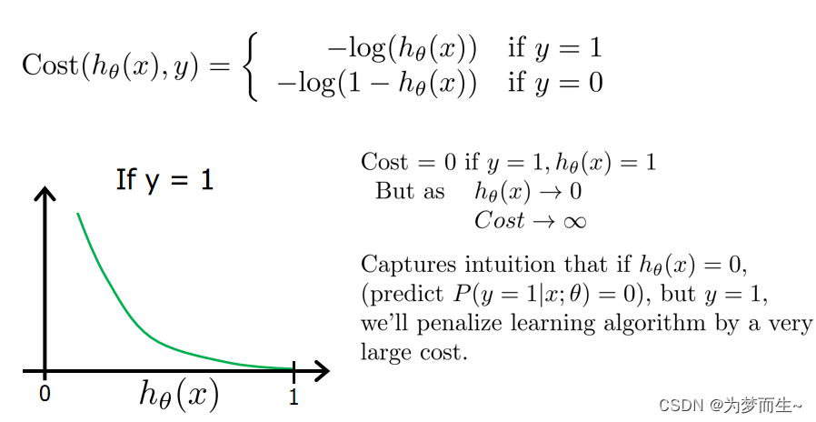
其原理是利用的正规公式:

实现过程也是相当于这个公式的计算过程
CostHistory=[]
def Cost_Function(X, Y, theta, m):
    sumOfErrors = 0
    for i in range(m):
        xi = X[i]
        hi = Hypothesis(theta, xi)
        if Y[i] == 1:
            error = Y[i] * math.log(hi)
        elif Y[i] == 0:
            error = (1 - Y[i]) * math.log(1 - hi)
        sumOfErrors += error
        CostHistory.append(sumOfErrors)
    const = -1 / m
    J = const * sumOfErrors

    #print('cost is ', J)
    return CostHistory
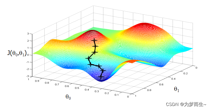
梯度下降
【机器学习基础】一元线性回归(适合初学者的保姆级文章)
【机器学习基础】多元线性回归(适合初学者的保姆级文章)
在这两篇文章中已经讲过了梯度下降的一些基本概念,如果不清楚的可以到前面看一下
代码定义梯度下降的方式如下:
def Gradient_Descent(X, Y, theta, m, alpha):
    new_theta = []
    constant = alpha / m
    for j in range(len(theta)):
        CFDerivative = Cost_Function_Derivative(X, Y, theta, j, m, alpha)
        new_theta_value = theta[j] - CFDerivative
        new_theta.append(new_theta_value)
    return new_theta
每次迭代,通过学习率与微分的计算,得到新的 θ \theta θ
迭代的策略这里使用的是牛顿法逻辑回归的实现,使用梯度下降来更新参数,同时使用二分法来逼近最优解。
def newton(X, Y, alpha, theta, num_iters):
    m = len(Y)
    for x in range(num_iters):
        new_theta = Gradient_Descent(X, Y, theta, m, alpha)
        theta = new_theta
        if x % 100 == 0:
            Cost_Function(X, Y, theta, m)
            print('theta ', theta)
            print('cost is ', Cost_Function(X, Y, theta, m))
    Declare_Winner(theta)
代码实现
from sklearn import preprocessing
from sklearn.linear_model import LogisticRegression
from sklearn.model_selection import train_test_split
from numpy import loadtxt, where
from pylab import scatter, show, legend, xlabel, ylabel
import math
import numpy as np
import pandas as pd
from pandas import DataFrame
import matplotlib.pyplot as plt


# 这是Sigmoid激活函数,用于将任何实数映射到介于0和1之间的值。
def Sigmoid(z):
    G_of_Z = float(1.0 / float((1.0 + math.exp(-1.0 * z))))
    return G_of_Z


# 这是预测函数,输入参数是参数向量theta和输入向量x,返回预测的概率。
def Hypothesis(theta, x):
    z = 0
    for i in range(len(theta)):
        z += x[i] * theta[i]
    return Sigmoid(z)


# 这是代价函数,输入参数是训练数据集X、标签Y、参数向量theta和样本数m,返回当前参数下的代价函数值和历史误差记录。
CostHistory=[]
def Cost_Function(X, Y, theta, m):
    sumOfErrors = 0
    for i in range(m):
        xi = X[i]
        hi = Hypothesis(theta, xi)
        if Y[i] == 1:
            error = Y[i] * math.log(hi)
        elif Y[i] == 0:
            error = (1 - Y[i]) * math.log(1 - hi)
        sumOfErrors += error
        CostHistory.append(sumOfErrors)
    const = -1 / m
    J = const * sumOfErrors

    #print('cost is ', J)
    return CostHistory


# 这是代价函数对第j个参数的导数,用于计算梯度下降中的梯度。
def Cost_Function_Derivative(X, Y, theta, j, m, alpha):
    sumErrors = 0
    for i in range(m):
        xi = X[i]
        xij = xi[j]
        hi = Hypothesis(theta, X[i])
        error = (hi - Y[i]) * xij
        sumErrors += error
    m = len(Y)
    constant = float(alpha) / float(m)
    J = constant * sumErrors
    return J


# 这是梯度下降算法的实现,用于更新参数向量theta。
def Gradient_Descent(X, Y, theta, m, alpha):
    new_theta = []
    constant = alpha / m
    for j in range(len(theta)):
        CFDerivative = Cost_Function_Derivative(X, Y, theta, j, m, alpha)
        new_theta_value = theta[j] - CFDerivative
        new_theta.append(new_theta_value)
    return new_theta


# 这是牛顿法逻辑回归的实现,使用梯度下降来更新参数,同时使用二分法来逼近最优解。
def newton(X, Y, alpha, theta, num_iters):
    m = len(Y)
    for x in range(num_iters):
        new_theta = Gradient_Descent(X, Y, theta, m, alpha)
        theta = new_theta
        if x % 100 == 0:
            Cost_Function(X, Y, theta, m)
            print('theta ', theta)
            print('cost is ', Cost_Function(X, Y, theta, m))
    Declare_Winner(theta)


# 该函数主要用于确定训练好的逻辑回归模型(这里命名为clf)对测试集的预测结果,并返回一个赢家(预测准确率更高的模型)。
def Declare_Winner(theta):
    score = 0
    winner = ""
    scikit_score = clf.score(X_test, Y_test)
    length = len(X_test)
    for i in range(length):
        prediction = round(Hypothesis(X_test[i], theta))
        answer = Y_test[i]
        if prediction == answer:
            score += 1
    my_score = float(score) / float(length)
min_max_scaler = preprocessing.MinMaxScaler(feature_range=(-1, 1))

x_input1, x_input2, Y = np.genfromtxt('dataset3.txt', unpack=True, delimiter=',')
print(x_input1.shape)
print(x_input2.shape)
print(Y.shape)
X = np.column_stack((x_input1, x_input2))

X = min_max_scaler.fit_transform(X)

X_train, X_test, Y_train, Y_test = train_test_split(X, Y, test_size=0.33)

clf= LogisticRegression()
clf.fit(X_train, Y_train)
print('Acuraccy is: ', (clf.score(X_test, Y_test) * 100))
pos = where(Y == 1)
neg = where(Y == 0)
scatter(X[pos, 0], X[pos, 1], marker='o', c='b')
scatter(X[neg, 0], X[neg, 1], marker='x', c='g')
xlabel('score 1')
ylabel('score 2')
legend(['0', '1'])


initial_theta = [0, 0]
alpha = 0.01
iterations = 100
m = len(Y)
mycost=Cost_Function(X,Y,initial_theta,m)
mycost=np.asarray(mycost)
print(mycost.shape)
plt.figure()
plt.plot(range(iterations),mycost)
newton(X,Y,alpha,initial_theta,iterations)
# print("theta is: ",my_theta)
plt.show()
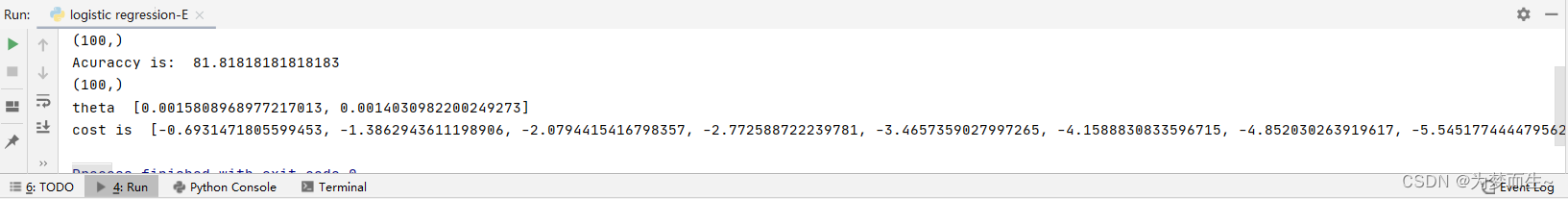
效果展示
首先是基于数据集做出的散点图,并标记出了正例和负例

对于该散点图,可以做出一条分割正负样本的直线

下面是程序的一些输出:


 被折叠的 条评论
为什么被折叠?
被折叠的 条评论
为什么被折叠?
 到【灌水乐园】发言


