


 本文详细介绍了非线性最小二乘问题的数值方法,从牛顿迭代法出发,探讨了高斯-牛顿法在解决实际问题中的应用,包括符号计算和Python实现的实例计算过程。
Title: 非线性最小二乘问题的数值方法 —— 从牛顿迭代法到高斯-牛顿法 (实例篇 V)
姊妹博文
非线性最小二乘问题的数值方法 —— 从牛顿迭代法到高斯-牛顿法 (I)
非线性最小二乘问题的数值方法 —— 从牛顿迭代法到高斯-牛顿法 (II)
非线性最小二乘问题的数值方法 —— 从牛顿迭代法到高斯-牛顿法 (III)
非线性最小二乘问题的数值方法 —— 从牛顿迭代法到高斯-牛顿法 (IV)
↑ \uparrow ↑ 理论部分
↓ \downarrow ↓ 实例部分
非线性最小二乘问题的数值方法 —— 从牛顿迭代法到高斯-牛顿法 (实例篇 V) ⟵ \longleftarrow ⟵ 本篇
0.前言
本篇博文作为对前述 “非线性最小二乘问题的数值方法 —— 从牛顿迭代法到高斯-牛顿法” 的实践扩展, 理论部分参见前述博文, 此处不再重复.
1. 最优问题实例
m i n i m i z e g ( x ) = 1 2 ∥ r ( x ) ∥ 2 2 = 1 2 ∑ i = 1 3 r i ( x ) 2 (I-1) {\rm minimize}\quad {g}(\mathbf{x}) = \frac{1}{2}\|\mathbf{r}(\mathbf{x})\|_2^2 = \frac{1}{2}\sum_{i=1}^{3} r_i(\mathbf{x})^2 \tag{I-1} minimizeg(x)=21∥r(x)∥22=21i=1∑3ri(x)2(I-1)
其中
x = [ x 1 , x 2 ] T \mathbf{x} = \begin{bmatrix} x_1, x_2 \end{bmatrix}^{\small\rm T} x=[x1,x2]T
r ( x ) = [ r 1 ( x ) , r 2 ( x ) , r 3 ( x ) ] T \mathbf{r}(\mathbf{x}) = \begin{bmatrix} r_1(\mathbf{x}), \, r_2(\mathbf{x}) ,\,r_3(\mathbf{x}) \end{bmatrix}^{\small\rm T} r(x)=[r1(x),r2(x),r3(x)]T
r 1 ( x ) = sin x 1 − 0.4 r_1(\mathbf{x}) = \sin x_1 -0.4 r1(x)=sinx1−0.4
r 2 ( x ) = cos x 2 + 0.8 r_2(\mathbf{x}) = \cos x_2 + 0.8 r2(x)=cosx2+0.8
r 3 ( x ) = x 1 2 + x 2 2 − 1 r_3(\mathbf{x}) = \sqrt{x_1^2 +x_2^2} -1 r3(x)=x12+x22−1
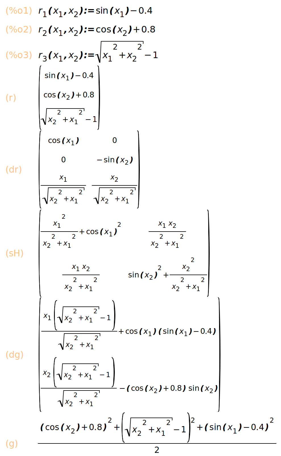
2. 符号计算
Maxima 符号运算代码:
(%i10) r_1(x_1,x_2) := sin(x_1)-0.4;
r_2(x_1,x_2) :=cos(x_2)+0.8;
r_3(x_1,x_2) := sqrt((x_1)^2 +(x_2)^2)-1;
r: matrix([r_1(x_1,x_2)], [r_2(x_1,x_2)], [r_3(x_1,x_2)]);
dr: matrix([diff(r_1(x_1,x_2), x_1), diff(r_1(x_1,x_2), x_2)], [diff(r_2(x_1,x_2), x_1), diff(r_2(x_1,x_2), x_2)], [diff(r_3(x_1,x_2), x_1), diff(r_3(x_1,x_2), x_2)]);
sH: transpose(dr) . dr;
dg: transpose(dr) . r;
g : (1/2) * (r_1(x_1,x_2)^2+r_2(x_1,x_2)^2+r_3(x_1,x_2)^2);
dg: ratexpand(matrix([diff(g,x_1)], [diff(g,x_2)]));
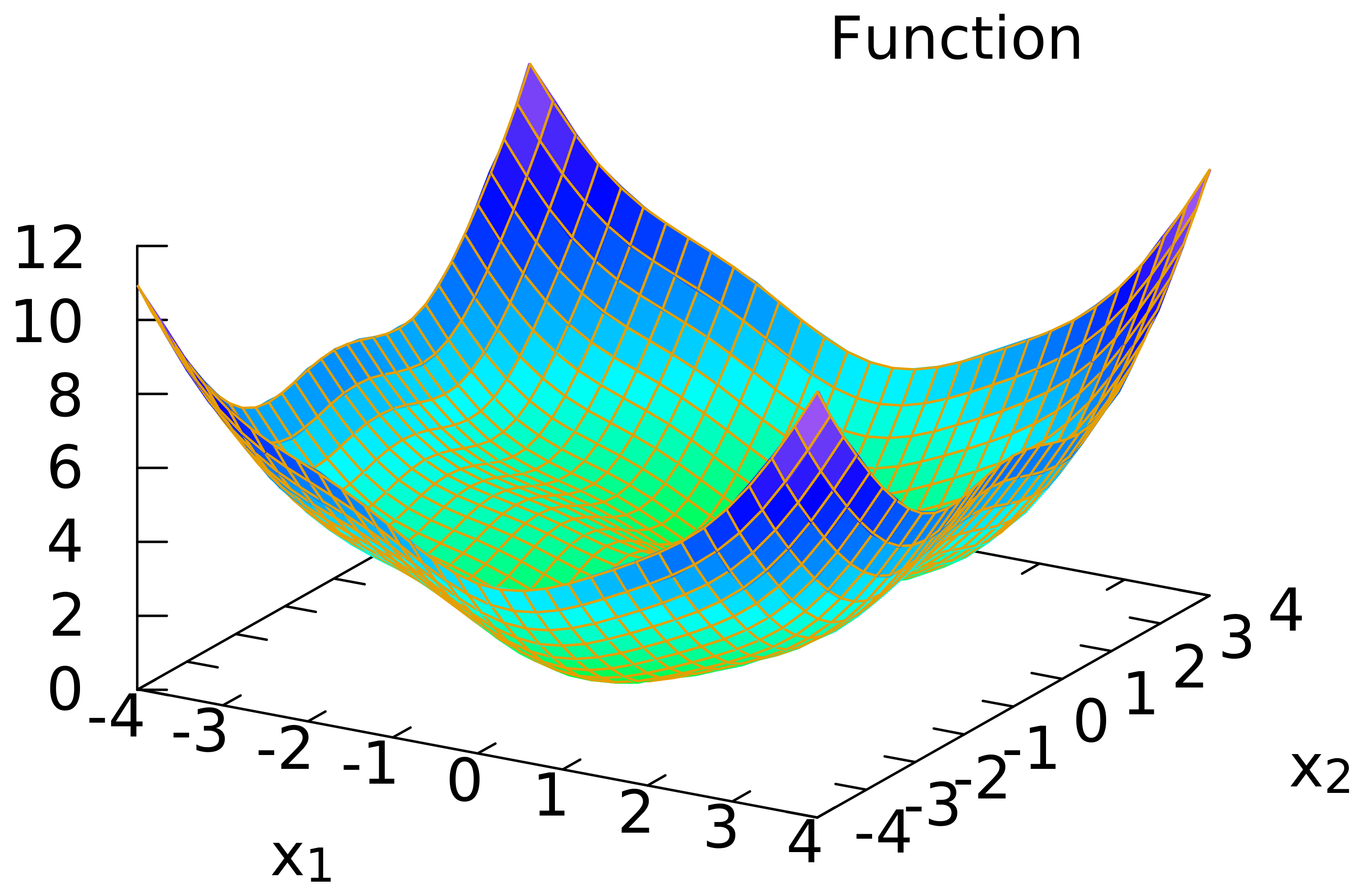
plot3d(g, [x_1,-4,4], [x_2,-4,4]);
(%o1) r_1(x_1,x_2):=sin(x_1)-0.4
(%o2) r_2(x_1,x_2):=cos(x_2)+0.8
(%o3) r_3(x_1,x_2):=sqrt(x_1^2+x_2^2)-1
(r) matrix(
[sin(x_1)-0.4],
[cos(x_2)+0.8],
[sqrt(x_2^2+x_1^2)-1]
)
(dr) matrix(
[cos(x_1), 0],
[0, -sin(x_2)],
[x_1/sqrt(x_2^2+x_1^2), x_2/sqrt(x_2^2+x_1^2)]
)
(sH) matrix(
[x_1^2/(x_2^2+x_1^2)+cos(x_1)^2, (x_1*x_2)/(x_2^2+x_1^2)],
[(x_1*x_2)/(x_2^2+x_1^2), sin(x_2)^2+x_2^2/(x_2^2+x_1^2)]
)
(dg) matrix(
[(x_1*(sqrt(x_2^2+x_1^2)-1))/sqrt(x_2^2+x_1^2)+cos(x_1)*(sin(x_1)-0.4)],
[(x_2*(sqrt(x_2^2+x_1^2)-1))/sqrt(x_2^2+x_1^2)-(cos(x_2)+0.8)*sin(x_2)]
)
(g) ((cos(x_2)+0.8)^2+(sqrt(x_2^2+x_1^2)-1)^2+(sin(x_1)-0.4)^2)/2
rat: replaced -0.4 by -2/5 = -0.4
rat: replaced 0.8 by 4/5 = 0.8
(dg) matrix(
[-x_1/sqrt(x_2^2+x_1^2)+cos(x_1)*sin(x_1)-(2*cos(x_1))/5+x_1],
[-cos(x_2)*sin(x_2)-(4*sin(x_2))/5-x_2/sqrt(x_2^2+x_1^2)+x_2]
)
(%o10) ["/tmp/maxout347947.gnuplot_pipes"]
3. 高斯-牛顿法计算
from mpl_toolkits.mplot3d import axes3d
import matplotlib.pyplot as plt
import numpy as np
from numpy.linalg import inv, det
from math import cos
from math import sin
from math import sqrt
from math import pow
# multiplication of two matrixs
def multiply_matrix(A, B):
if A.shape[1] == B.shape[0]:
C = np.zeros((A.shape[0], B.shape[1]), dtype = float)
[rows, cols] = C.shape
for row in range(rows):
for col in range(cols):
for elt in range(len(B)):
C[row, col] += A[row, elt] * B[elt, col]
return C
else:
return "Cannot multiply A and B. Please check whether the dimensions of the inputs are compatible."
# g(x) = (1/2) ||r(x)||_2^2
def g(x_1, x_2):
return ( pow(sin(x_1)-0.4, 2)+ pow(cos(x_2)+0.8, 2) + pow(sqrt(pow(x_2,2)+pow(x_1,2))-1, 2) ) /2
# r(x) = [r_1, r_2, r_3]^{T}
def r(x_1, x_2):
return np.array([[sin(x_1)-0.4],
[cos(x_2)+0.8],
[sqrt(pow(x_1,2)+pow(x_2,2))-1]])
# \partial r(x) / \partial x
def dr(x_1, x_2):
if sqrt(pow(x_2,2)+pow(x_1,2)) == 0: ## 人为设置
return np.array([[cos(x_1), 0],
[0, -sin(x_2)],
[0, 0]])
else:
return np.array([[cos(x_1), 0],
[0, -sin(x_2)],
[x_1/sqrt(pow(x_2,2)+pow(x_1,2)), x_2/sqrt(pow(x_2,2)+pow(x_1,2))]])
# Simplified Hessian matrix in Gauss-Newton method, refer to eq. (IV-1-2)
def sH(x_1, x_2):
return multiply_matrix(np.transpose(dr(x_1, x_2)), dr(x_1, x_2))
# \nabla g(x_1, x_2), refer to eq. (III-1-2)
def dg(x_1, x_2):
return multiply_matrix(np.transpose(dr(x_1, x_2)), r(x_1, x_2))
def gauss_newton_method(x_1, x_2, epsilon, max_iter):
iter = 0
array_x_1 = []
array_x_2 = []
array_x_3 = []
new_x = np.matrix([[0],[0]])
while iter < max_iter:
array_x_1.append(x_1)
array_x_2.append(x_2)
array_x_3.append(g(x_1, x_2))
# print("iter: %d"%iter)
# print("x_1: %f"%x_1)
# print("x_2: %f"%x_2)
# print("g: %f"%g(x_1, x_2))
# print("sH:")
# print(sH(x_1, x_2))
# print("inv(sH):")
# print(inv(sH(x_1, x_2)))
sH_i = sH(x_1, x_2)
if det(sH_i) == 0:
print("The simplified Hessian matrix in Guass-Newton Method is singular.")
break
else:
inv_sH_i = inv(sH_i)
dg_i = dg(x_1, x_2)
new_x = np.matrix([[x_1], [x_2]]) - multiply_matrix(inv_sH_i, dg_i)
update_distance = sqrt(pow(x_1-new_x[0,0], 2) + pow(x_2-new_x[1,0], 2))
# print("update_distance: %f"%update_distance)
if update_distance < epsilon:
break
iter += 1
x_1 = new_x[0,0]
x_2 = new_x[1,0]
return array_x_1, array_x_2, array_x_3
def result_plot(trajectory):
fig = plt.figure()
ax3 = plt.axes(projection='3d')
xx = np.arange(-5,5,0.1)
yy = np.arange(-4,4,0.1)
X, Y = np.meshgrid(xx, yy)
Z = np.zeros((X.shape[0], Y.shape[1]), dtype = float)
for i in range(X.shape[0]):
for j in range(Y.shape[1]):
Z[i,j] = g(X[0,j], Y[i,0])
ax3.plot_surface(X, Y, Z, rstride = 1, cstride = 1, cmap='rainbow', alpha=0.25)
ax3.contour(X, Y, Z, offset=-1, cmap = 'rainbow')
ax3.plot(trajectory[0], trajectory[1], trajectory[2], "r--")
offset_data = -1*np.ones(len(trajectory[0]))
ax3.plot(trajectory[0], trajectory[1], offset_data,'k--')
ax3.set_title('Guass-Newton Method (Initial point [%.1f, %.1f])' %(trajectory[0][0], trajectory[1][0]))
file_name_prefix = "./gauss_newton"
file_extension = ".png"
file_name = f"{file_name_prefix}_{trajectory[0][0]}_{trajectory[1][0]}{file_extension}"
print(file_name)
plt.draw()
plt.savefig(file_name)
if __name__ == "__main__":
test_data = np.array([[4.9, 3.9], [-2.9, 1.9], [0.1, -0.1], [-0.1, 0.1], [0,-3.8],[1,2.5], [0,0]])
for inital_data in test_data:
print("\nInitial point:")
print(inital_data)
x_1 = inital_data[0]
x_2 = inital_data[1]
epsilon = 1e-10
max_iter = 1000
trajectory = gauss_newton_method(x_1, x_2, epsilon, max_iter)
result_plot(trajectory)
得到的结果:
| 测试显示 | 测试显示 |
|---|---|
 |  |
 |  |
 |  |
4. 结论
围绕一个最小二乘问题实例, 利用 Maxima 进行了公式推导, 利用 Python 进行了数值计算和结果显示.
(如有问题请指出, 谢谢! )


 1469
1469

 被折叠的 条评论
为什么被折叠?
被折叠的 条评论
为什么被折叠?
 到【灌水乐园】发言


