机器学习--化直为曲：逻辑斯蒂回归

化直为曲：逻辑斯蒂回归

1. 逻辑斯蒂回归简介

：逻辑斯蒂回归是一个较为简单的分类器，既可以处理二分类问题也可以处理多分类问题。它通过一个非线性函数对数据样本的类别进行学习，可以看作对样本属于某一类别的概率进行回归，已经被标定为某一类别标签的训练样本 ，我们就认为是它属于该类别的概率为1，属于其他的概率为0.然后将训练好的模型应用于新的样本，就可以输出该样本是每个类别的概率分别是多少，选择概率最大的类别作为最终的分类结果。

2. 逻辑斯蒂回归任务类型

：通常用来处理二分类问题或多分类问题。与SVM直接在空间上进行划分，并给出硬性指标的类别不同，逻辑斯蒂回归可以将每个样本点的特征向量映射为其是否归属某一类别的一个概率值。

3.逻辑斯蒂回归的基本原理

：逻辑斯蒂回归是一个分类器，通常被用于解决分类问题。首先要介绍回归问题和分类问题。
分类问题：根据样本特征预测其属于哪一个类别。类别是离散值
回归问题：根据输入的样本特征预测出一个连续值的输出。

4.代码实现

该代码的例子利用了scikit-learn中自带的数据集digits，即手写数字的数据集。该数据集包含1797个0~9的手写字体，这里只取0和1 作为任务数据集。主要任务是通过逻辑斯蒂回归的方法，将一个手写字体数字图像分类到正确的数值。

import numpy as np
from sklearn.datasets import load_digits
import matplotlib.pyplot as plt
from sklearn.linear_model import LogisticRegression
from sklearn.model_selection import train_test_split
#加载数据
digits=load_digits()
data=digits.data
target=digits.target
#打印数据集大小
print(digits)
print(data.shape)
print(target.shape)
#找到0和1 手写体数据的位置
where_0=np.where(target==0)
where_1=np.where(target==1)
print(where_1)
print(where_0)
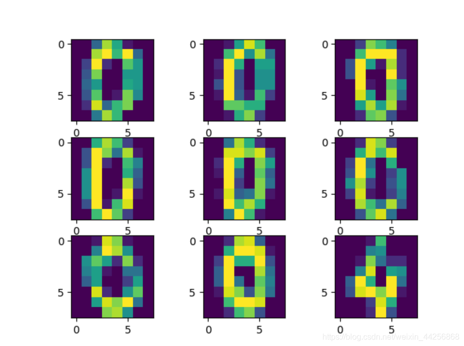
#显示前9个不同写法的0和1
# for i in range(9):
#     plt.subplot(3,3,i+1)
#     plt.imshow(digits.data[where_0[0][i],:].reshape([8,8]))
# plt.show()
#
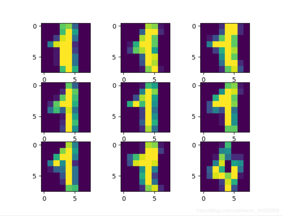
# for i in range(9):
#     plt.subplot(3,3,i+1)
#     plt.imshow(digits.data[where_1[0][i],:].reshape([8,8]))
# plt.show()
#制作后面用于分类任务的0和1手写体数据集，并打印出数据集大小
zero_data=data[where_0[0],:]
ones_data=data[where_1[0],:]
print(zero_data.shape)
print(ones_data.shape)
#生成样本输入和对应的真实答案
X=np.concatenate((zero_data,ones_data),axis=0)
y=np.array([0]*zero_data.shape[0]+[1]*ones_data.shape[0])
print(y.shape)
#将训练集随机重排
order=np.random.permutation(X.shape[0])
X=X[order,:]
y=y[order]
#划分训练集和测试集
X_train,X_test,y_train,y_test=train_test_split(X,y,test_size=0.4,random_state=42)
print(X_train.shape,y_train.shape)
clf=LogisticRegression(random_state=42,solver='lbfgs',multi_class='multinomial',max_iter=10000,tol=1e-8,C=50)
#训练逻辑斯蒂回归模型
clf.fit(X_train,y_train)
#打印训练集和测试集精度
print(clf.score(X_train,y_train))
print(clf.score(X_test,y_test))
#测试集的预测类别结果
pred=clf.predict(X_test)
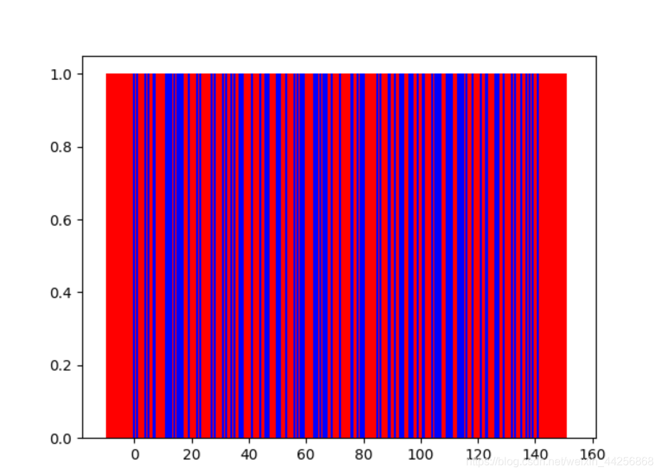
#测试集的预测概率
y_proba=clf.predict_proba(X_test)[:,1]
#将实际概率与预测概率作图显示
# plt.bar(range(len(y_proba)),+y_proba,width=20,facecolor='red')
# plt.bar(range(len(y_test)),+y_test,facecolor='blue')
# plt.show()
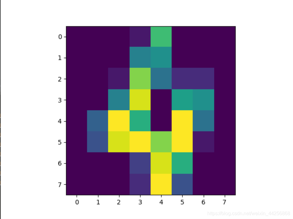
four=data[np.where(target==4)[0][0],:]
plt.imshow(four.reshape([8,8]))
plt.show()
print(clf.predict(four.reshape(1,64)))
print(clf.predict_proba(four.reshape(1,64)))

5,实验结果