T9 TensorFlow入门实战——猫狗识别2-优快云博客

本文链接：https://blog.youkuaiyun.com/weixin_43934209/article/details/146219751

🍨 本文為🔗365天深度學習訓練營中的學習紀錄博客
🍖 原作者：K同学啊 | 接輔導、項目定制

一、前期准备

1. 导入数据

# Import the required libraries
import numpy as np
import PIL,pathlib
from PIL import Image
import matplotlib.pyplot as plt
import numpy as np
import tensorflow as tf
from tensorflow import keras
from tensorflow.keras import layers, models, Input
from tensorflow.keras.models import Model
from tensorflow.keras.layers import Conv2D, MaxPooling2D, Dense, Flatten, Dropout
from tqdm import tqdm
import tensorflow.keras.backend as K
from datetime import datetime



# load the data
data_dir = './data/365-7-data/'
data_dir = pathlib.Path(data_dir)

data_paths = list(data_dir.glob('*'))
classeNames = [str(path).split("\\")[2] for path in data_paths]
classeNames

2. 查看数据

image_count = len(list(data_dir.glob('*/*')))

print("图片总数为：",image_count)

二、数据预处理

1. 加载数据

# Data loading and preprocessing
batch_size = 64
img_height = 224
img_width = 224

"""
关于image_dataset_from_directory()的详细介绍可以参考文章：https://mtyjkh.blog.youkuaiyun.com/article/details/117018789
"""
train_ds = tf.keras.preprocessing.image_dataset_from_directory(
    data_dir,
    validation_split=0.2,
    subset="training",
    seed=12,
    image_size=(img_height, img_width),
    batch_size=batch_size)

"""
关于image_dataset_from_directory()的详细介绍可以参考文章：https://mtyjkh.blog.youkuaiyun.com/article/details/117018789
"""
val_ds = tf.keras.preprocessing.image_dataset_from_directory(
    data_dir,
    validation_split=0.2,
    subset="validation",
    seed=12,
    image_size=(img_height, img_width),
    batch_size=batch_size)

class_names = train_ds.class_names
print(class_names)

2. 可视化数据

# Visualize the data
plt.figure(figsize=(15, 10))

for images, labels in train_ds.take(1):
    for i in range(8):
        ax = plt.subplot(5, 8, i + 1)

        plt.imshow(images[i].numpy().astype("uint8"))
        plt.title(class_names[np.argmax(labels[i])])
        
        plt.axis("off")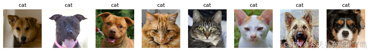

# Check the shape of the data
for image_batch, labels_batch in train_ds:
    print(image_batch.shape)
    print(labels_batch.shape)
    break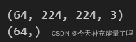

3. 配置数据集

AUTOTUNE = tf.data.AUTOTUNE

def preprocess_image(image,label):
    return (image/255.0,label)

# Normalize the data
train_ds = train_ds.map(preprocess_image, num_parallel_calls=AUTOTUNE)
val_ds   = val_ds.map(preprocess_image, num_parallel_calls=AUTOTUNE)

train_ds = train_ds.cache().shuffle(1000).prefetch(buffer_size=AUTOTUNE)
val_ds   = val_ds.cache().prefetch(buffer_size=AUTOTUNE)

三、训练模型

1. 构建VGG-16网络模型

def VGG16(nb_classes, input_shape):
    input_tensor = Input(shape=input_shape)
    # 1st block
    x = Conv2D(64, (3,3), activation='relu', padding='same',name='block1_conv1')(input_tensor)
    x = Conv2D(64, (3,3), activation='relu', padding='same',name='block1_conv2')(x)
    x = MaxPooling2D((2,2), strides=(2,2), name = 'block1_pool')(x)
    # 2nd block
    x = Conv2D(128, (3,3), activation='relu', padding='same',name='block2_conv1')(x)
    x = Conv2D(128, (3,3), activation='relu', padding='same',name='block2_conv2')(x)
    x = MaxPooling2D((2,2), strides=(2,2), name = 'block2_pool')(x)
    # 3rd block
    x = Conv2D(256, (3,3), activation='relu', padding='same',name='block3_conv1')(x)
    x = Conv2D(256, (3,3), activation='relu', padding='same',name='block3_conv2')(x)
    x = Conv2D(256, (3,3), activation='relu', padding='same',name='block3_conv3')(x)
    x = MaxPooling2D((2,2), strides=(2,2), name = 'block3_pool')(x)
    # 4th block
    x = Conv2D(512, (3,3), activation='relu', padding='same',name='block4_conv1')(x)
    x = Conv2D(512, (3,3), activation='relu', padding='same',name='block4_conv2')(x)
    x = Conv2D(512, (3,3), activation='relu', padding='same',name='block4_conv3')(x)
    x = MaxPooling2D((2,2), strides=(2,2), name = 'block4_pool')(x)
    # 5th block
    x = Conv2D(512, (3,3), activation='relu', padding='same',name='block5_conv1')(x)
    x = Conv2D(512, (3,3), activation='relu', padding='same',name='block5_conv2')(x)
    x = Conv2D(512, (3,3), activation='relu', padding='same',name='block5_conv3')(x)
    x = MaxPooling2D((2,2), strides=(2,2), name = 'block5_pool')(x)
    # full connection
    x = Flatten()(x)
    x = Dense(4096, activation='relu',  name='fc1')(x)
    x = Dense(4096, activation='relu', name='fc2')(x)
    output_tensor = Dense(nb_classes, activation='softmax', name='predictions')(x)

    model = Model(input_tensor, output_tensor)
    return model

model=VGG16(len(class_names), (img_width, img_height, 3))
model.summary()

Model: "model"
_________________________________________________________________
 Layer (type)                Output Shape              Param #   
=================================================================
 input_1 (InputLayer)        [(None, 224, 224, 3)]     0         
                                                                 
 block1_conv1 (Conv2D)       (None, 224, 224, 64)      1792      
                                                                 
 block1_conv2 (Conv2D)       (None, 224, 224, 64)      36928     
                                                                 
 block1_pool (MaxPooling2D)  (None, 112, 112, 64)      0         
                                                                 
 block2_conv1 (Conv2D)       (None, 112, 112, 128)     73856     
                                                                 
 block2_conv2 (Conv2D)       (None, 112, 112, 128)     147584    
                                                                 
 block2_pool (MaxPooling2D)  (None, 56, 56, 128)       0         
                                                                 
 block3_conv1 (Conv2D)       (None, 56, 56, 256)       295168    
                                                                 
 block3_conv2 (Conv2D)       (None, 56, 56, 256)       590080    
                                                                 
 block3_conv3 (Conv2D)       (None, 56, 56, 256)       590080    
                                                                 
 block3_pool (MaxPooling2D)  (None, 28, 28, 256)       0         
                                                                 
 block4_conv1 (Conv2D)       (None, 28, 28, 512)       1180160   
                                                                 
 block4_conv2 (Conv2D)       (None, 28, 28, 512)       2359808   
                                                                 
 block4_conv3 (Conv2D)       (None, 28, 28, 512)       2359808   
                                                                 
 block4_pool (MaxPooling2D)  (None, 14, 14, 512)       0         
                                                                 
 block5_conv1 (Conv2D)       (None, 14, 14, 512)       2359808   
                                                                 
 block5_conv2 (Conv2D)       (None, 14, 14, 512)       2359808   
                                                                 
 block5_conv3 (Conv2D)       (None, 14, 14, 512)       2359808   
                                                                 
 block5_pool (MaxPooling2D)  (None, 7, 7, 512)         0         
                                                                 
 flatten (Flatten)           (None, 25088)             0         
                                                                 
 fc1 (Dense)                 (None, 4096)              102764544 
                                                                 
 fc2 (Dense)                 (None, 4096)              16781312  
                                                                 
 predictions (Dense)         (None, 2)                 8194      
                                                                 
=================================================================
Total params: 134268738 (512.19 MB)
Trainable params: 134268738 (512.19 MB)
Non-trainable params: 0 (0.00 Byte)
_________________________________________________________________

2. 编译模型

model.compile(optimizer="adam",
              loss     ='sparse_categorical_crossentropy',
              metrics  =['accuracy'])

3. 训练模型

与上次代码相比，此处只记录了最后一个 batch 的 loss 和 accuracy

epochs = 10
lr     = 1e-4

# 记录训练数据，方便后面的分析
history_train_loss     = []
history_train_accuracy = []
history_val_loss       = []
history_val_accuracy   = []

for epoch in range(epochs):
    train_total = len(train_ds)
    val_total   = len(val_ds)
    
    """
    total：预期的迭代数目
    ncols：控制进度条宽度
    mininterval：进度更新最小间隔，以秒为单位（默认值：0.1）
    """
    with tqdm(total=train_total, desc=f'Epoch {epoch + 1}/{epochs}',mininterval=1,ncols=100) as pbar:
        lr = lr*0.92
        K.set_value(model.optimizer.learning_rate, lr)

        train_loss     = []
        train_accuracy = []
        
        for image,label in train_ds:   
            """
            训练模型，简单理解train_on_batch就是：它是比model.fit()更高级的一个用法

            想详细了解 train_on_batch 的同学，
            可以看看我的这篇文章：https://www.yuque.com/mingtian-fkmxf/hv4lcq/ztt4gy
            """
             # 这里生成的是每一个batch的acc与loss
            history = model.train_on_batch(image,label)
            
            train_loss.append(history[0])
            train_accuracy.append(history[1])
            
            pbar.set_postfix({"train_loss": "%.4f"%history[0],
                              "train_acc":"%.4f"%history[1],
                              "lr": K.get_value(model.optimizer.lr)})
            pbar.update(1)
            
        history_train_loss.append(np.mean(train_loss))
        history_train_accuracy.append(np.mean(train_accuracy))
            
    print('开始验证！')
    
    with tqdm(total=val_total, desc=f'Epoch {epoch + 1}/{epochs}',mininterval=0.3,ncols=100) as pbar:

        val_loss     = []
        val_accuracy = []
        for image,label in val_ds:      
            # 这里生成的是每一个batch的acc与loss
            history = model.test_on_batch(image,label)
            
            val_loss.append(history[0])
            val_accuracy.append(history[1])
            
            pbar.set_postfix({"val_loss": "%.4f"%history[0],
                              "val_acc":"%.4f"%history[1]})
            pbar.update(1)
        history_val_loss.append(np.mean(val_loss))
        history_val_accuracy.append(np.mean(val_accuracy))
            
    print('结束验证！')
    print("验证loss为：%.4f"%np.mean(val_loss))
    print("验证准确率为：%.4f"%np.mean(val_accuracy))

Epoch 1/10: 100%|███| 43/43 [53:47<00:00, 75.05s/it, train_loss=0.6444, train_acc=0.6094, lr=9.2e-5]
开始验证！
Epoch 1/10: 100%|██████████████████| 11/11 [04:23<00:00, 23.91s/it, val_loss=0.7455, val_acc=0.5750]
结束验证！
验证loss为：0.7126
验证准确率为：0.5878
Epoch 2/10: 100%|██| 43/43 [51:41<00:00, 72.12s/it, train_loss=0.5205, train_acc=0.7500, lr=8.46e-5]
开始验证！
Epoch 2/10: 100%|██████████████████| 11/11 [02:56<00:00, 16.07s/it, val_loss=0.4389, val_acc=0.8250]
结束验证！
验证loss为：0.4533
验证准确率为：0.7852
Epoch 3/10: 100%|█| 43/43 [1:17:38<00:00, 108.35s/it, train_loss=0.1626, train_acc=0.9375, lr=7.79e-
开始验证！
Epoch 3/10: 100%|██████████████████| 11/11 [06:28<00:00, 35.31s/it, val_loss=0.1998, val_acc=0.9000]
结束验证！
验证loss为：0.2175
验证准确率为：0.9128
Epoch 4/10: 100%|█| 43/43 [1:33:29<00:00, 130.46s/it, train_loss=0.1484, train_acc=0.9688, lr=7.16e-
开始验证！
Epoch 4/10: 100%|██████████████████| 11/11 [05:39<00:00, 30.88s/it, val_loss=0.1060, val_acc=0.9500]
结束验证！
验证loss为：0.1086
验证准确率为：0.9514
Epoch 5/10: 100%|█| 43/43 [1:40:47<00:00, 140.63s/it, train_loss=0.1030, train_acc=0.9844, lr=6.59e-
开始验证！
Epoch 5/10: 100%|██████████████████| 11/11 [06:32<00:00, 35.72s/it, val_loss=0.0587, val_acc=0.9750]
结束验证！
验证loss为：0.0896
验证准确率为：0.9622
Epoch 6/10: 100%|█| 43/43 [2:54:04<00:00, 242.90s/it, train_loss=0.0301, train_acc=0.9844, lr=6.06e-
开始验证！
Epoch 6/10: 100%|██████████████████| 11/11 [06:34<00:00, 35.89s/it, val_loss=0.0461, val_acc=0.9750]
结束验证！
验证loss为：0.0658
验证准确率为：0.9722
Epoch 7/10: 100%|█| 43/43 [1:33:37<00:00, 130.63s/it, train_loss=0.0069, train_acc=1.0000, lr=5.58e-
开始验证！
Epoch 7/10: 100%|██████████████████| 11/11 [04:33<00:00, 24.85s/it, val_loss=0.0428, val_acc=0.9750]
结束验证！
验证loss为：0.0478
验证准确率为：0.9864
Epoch 8/10: 100%|█| 43/43 [1:02:40<00:00, 87.46s/it, train_loss=0.0073, train_acc=1.0000, lr=5.13e-5
开始验证！
Epoch 8/10: 100%|██████████████████| 11/11 [04:01<00:00, 21.98s/it, val_loss=0.0630, val_acc=0.9750]
结束验证！
验证loss为：0.0946
验证准确率为：0.9665
Epoch 9/10: 100%|██| 43/43 [58:40<00:00, 81.88s/it, train_loss=0.0070, train_acc=1.0000, lr=4.72e-5]
开始验证！
Epoch 9/10: 100%|██████████████████| 11/11 [04:03<00:00, 22.12s/it, val_loss=0.0256, val_acc=0.9750]
结束验证！
验证loss为：0.0308
验证准确率为：0.9920
Epoch 10/10: 100%|█| 43/43 [57:32<00:00, 80.30s/it, train_loss=0.0033, train_acc=1.0000, lr=4.34e-5]
开始验证！
Epoch 10/10: 100%|█████████████████| 11/11 [03:36<00:00, 19.72s/it, val_loss=0.0332, val_acc=0.9750]
结束验证！
验证loss为：0.0478
验证准确率为：0.9835

四、模型评估

1. Loss与Accuracy图

epochs_range = range(epochs)

plt.figure(figsize=(12, 4))
plt.subplot(1, 2, 1)

plt.plot(epochs_range, history_train_accuracy, label='Training Accuracy')
plt.plot(epochs_range, history_val_accuracy, label='Validation Accuracy')
plt.legend(loc='lower right')
plt.title('Training and Validation Accuracy')
plt.xlabel(current_time)

plt.subplot(1, 2, 2)
plt.plot(epochs_range, history_train_loss, label='Training Loss')
plt.plot(epochs_range, history_val_loss, label='Validation Loss')
plt.legend(loc='upper right')
plt.title('Training and Validation Loss')
plt.show()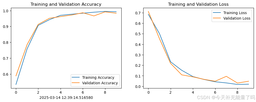

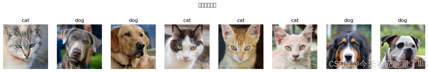
2. 预测

plt.figure(figsize=(18, 3))  # 图形的宽为18高为5
plt.suptitle("预测结果展示")

for images, labels in val_ds.take(1):
    for i in range(8):
        ax = plt.subplot(1,8, i + 1)  
        
        # 显示图片
        plt.imshow(images[i].numpy())
        
        # 需要给图片增加一个维度
        img_array = tf.expand_dims(images[i], 0) 
        
        # 使用模型预测图片中的人物
        predictions = model.predict(img_array)
        plt.title(class_names[np.argmax(predictions[0])])

        plt.axis("off")

五、数据增强与代码优化

1. 数据增强（提高模型泛化能力）

随机左右翻转 tf.image.random_flip_left_right
随机上下翻转 tf.image.random_flip_up_down
随机亮度变化 tf.image.random_brightness
随机对比度变化 tf.image.random_contrast

2. 代码模块化，增加可读性。

3. 增加BatchNormalization和Droupout防止过拟合。

# Import the required libraries
import numpy as np
import pathlib
import tensorflow as tf
import matplotlib.pyplot as plt
from datetime import datetime
from tensorflow.keras import layers, models, Input, backend as K
from tensorflow.keras.models import Model
from tensorflow.keras.optimizers.schedules import ExponentialDecay
from tensorflow.keras.layers import Conv2D, MaxPooling2D, Dense, Flatten, Dropout, BatchNormalization
from tqdm import tqdm

# Load dataset
data_dir = pathlib.Path('./data/365-7-data/')
batch_size = 32
img_height, img_width = 224, 224
AUTOTUNE = tf.data.AUTOTUNE

# Data augmentation
def augment_data(image, label):
    image = tf.image.random_flip_left_right(image)
    image = tf.image.random_flip_up_down(image)
    image = tf.image.random_brightness(image, max_delta=0.2)
    image = tf.image.random_contrast(image, lower=0.8, upper=1.2)
    image = image / 255.0  # Normalize
    return image, label

# Load train & validation datasets
train_ds = tf.keras.preprocessing.image_dataset_from_directory(
    data_dir, validation_split=0.2, subset="training", seed=12,
    image_size=(img_height, img_width), batch_size=batch_size)

val_ds = tf.keras.preprocessing.image_dataset_from_directory(
    data_dir, validation_split=0.2, subset="validation", seed=12,
    image_size=(img_height, img_width), batch_size=batch_size)

# Apply data augmentation to training set
train_ds = train_ds.map(augment_data, num_parallel_calls=AUTOTUNE).shuffle(1000).cache().prefetch(AUTOTUNE)
val_ds = val_ds.map(lambda x, y: (x / 255.0, y), num_parallel_calls=AUTOTUNE).cache().prefetch(AUTOTUNE)

class_names = train_ds.class_names
print("Classes:", class_names)

# Define model architecture
def VGG16(nb_classes, input_shape):
    input_tensor = Input(shape=input_shape)

    def conv_block(x, filters, block_name):
        x = Conv2D(filters, (3,3), activation='relu', padding='same', name=f'{block_name}_conv1')(x)
        x = BatchNormalization()(x)
        x = Conv2D(filters, (3,3), activation='relu', padding='same', name=f'{block_name}_conv2')(x)
        x = BatchNormalization()(x)
        x = MaxPooling2D((2,2), strides=(2,2), name=f'{block_name}_pool')(x)
        return x

    x = conv_block(input_tensor, 64, "block1")
    x = conv_block(x, 128, "block2")
    x = conv_block(x, 256, "block3")
    x = conv_block(x, 512, "block4")
    x = conv_block(x, 512, "block5")

    x = Flatten()(x)
    x = Dense(4096, activation='relu', name='fc1')(x)
    x = Dropout(0.5)(x)
    x = Dense(4096, activation='relu', name='fc2')(x)
    x = Dropout(0.5)(x)
    output_tensor = Dense(nb_classes, activation='softmax', name='predictions')(x)

    model = Model(input_tensor, output_tensor)
    return model

# Compile model with learning rate schedule
lr_schedule = ExponentialDecay(initial_learning_rate=1e-4, decay_steps=1000, decay_rate=0.92, staircase=True)
model = VGG16(len(class_names), (img_width, img_height, 3))
model.compile(optimizer=tf.keras.optimizers.Adam(learning_rate=lr_schedule),
              loss='sparse_categorical_crossentropy',
              metrics=['accuracy'])

model.summary()

# Training loop
epochs = 10
history_train_loss, history_train_accuracy = [], []
history_val_loss, history_val_accuracy = [], []

for epoch in range(epochs):
    train_loss, train_acc = [], []
    val_loss, val_acc = [], []

    print(f'\nEpoch {epoch + 1}/{epochs}')
    with tqdm(total=len(train_ds), desc='Training', ncols=100) as pbar:
        for image, label in train_ds:
            loss, acc = model.train_on_batch(image, label)
            train_loss.append(loss)
            train_acc.append(acc)
            pbar.set_postfix({"Loss": f"{loss:.4f}", "Acc": f"{acc:.4f}"})
            pbar.update(1)
    
    history_train_loss.append(np.mean(train_loss))
    history_train_accuracy.append(np.mean(train_acc))

    with tqdm(total=len(val_ds), desc='Validation', ncols=100) as pbar:
        for image, label in val_ds:
            loss, acc = model.test_on_batch(image, label)
            val_loss.append(loss)
            val_acc.append(acc)
            pbar.set_postfix({"Loss": f"{loss:.4f}", "Acc": f"{acc:.4f}"})
            pbar.update(1)
    
    history_val_loss.append(np.mean(val_loss))
    history_val_accuracy.append(np.mean(val_acc))

    print(f"Validation Loss: {np.mean(val_loss):.4f}, Accuracy: {np.mean(val_acc):.4f}")

# Plot training history
plt.figure(figsize=(12, 4))
plt.subplot(1, 2, 1)
plt.plot(range(epochs), history_train_accuracy, label='Training Acc')
plt.plot(range(epochs), history_val_accuracy, label='Validation Acc')
plt.legend(loc='lower right')
plt.title('Training & Validation Accuracy')

plt.subplot(1, 2, 2)
plt.plot(range(epochs), history_train_loss, label='Training Loss')
plt.plot(range(epochs), history_val_loss, label='Validation Loss')
plt.legend(loc='upper right')
plt.title('Training & Validation Loss')

plt.show()

# Test model on validation images
plt.figure(figsize=(18, 3))
plt.suptitle("Predictions")

for images, labels in val_ds.take(1):
    for i in range(8):
        ax = plt.subplot(1, 8, i + 1)
        plt.imshow(images[i].numpy())
        pred = model.predict(tf.expand_dims(images[i], 0))
        plt.title(class_names[np.argmax(pred[0])])
        plt.axis("off")