


- 🍨 本文為🔗365天深度學習訓練營 中的學習紀錄博客
- 🍖 原作者:K同学啊 | 接輔導、項目定制
一、前期准备
1. 导入数据
import tensorflow as tf
from tensorflow.keras import datasets, layers, models
import matplotlib.pyplot as plt

# 导入mnist数据,依次分别为训练集图片、训练集标签、测试集图片、测试集标签
(train_images, train_labels), (test_images, test_labels) = datasets.mnist.load_data()

2. 归一化
# Normalize pixel values to be between 0 and 1
train_images, test_images = train_images / 255.0, test_images / 255.0
# Check the shape of the data
print("Training data shape:", train_images.shape)
print("Training labels shape:", train_labels.shape)
print("Testing data shape:", test_images.shape)
print("Testing labels shape:", test_labels.shape)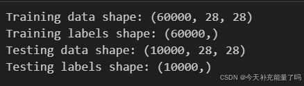
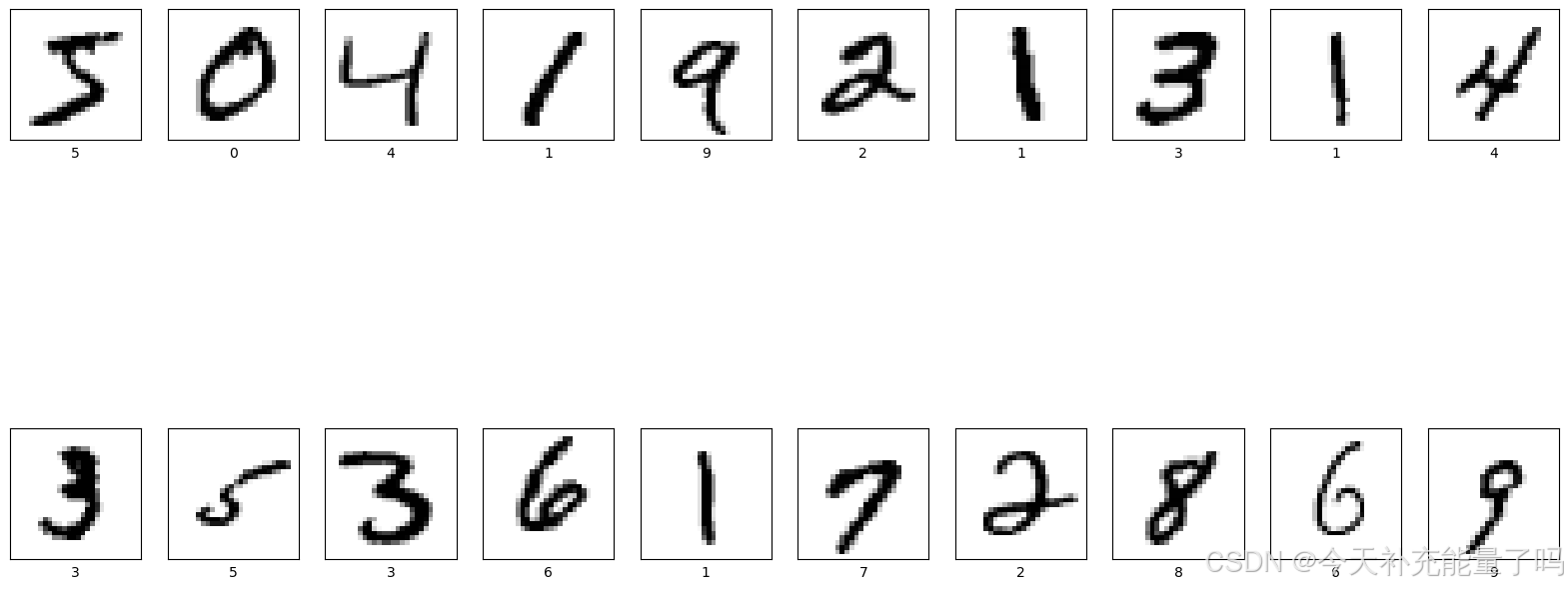
3. 可视化图片
# Plot the first 20 images
# 进行图像大小为20宽、10长的绘图(单位为英寸inch)
plt.figure(figsize=(20,10))
# 遍历MNIST数据集下标数值0~49
for i in range(20):
    # 将整个figure分成2行10列,绘制第i+1个子图。
    plt.subplot(2,10,i+1)
    # 设置不显示x轴刻度
    plt.xticks([])
    # 设置不显示y轴刻度
    plt.yticks([])
    # 设置不显示子图网格线
    plt.grid(False)
    # 图像展示,cmap为颜色图谱,"plt.cm.binary"为matplotlib.cm中的色表
    plt.imshow(train_images[i], cmap=plt.cm.binary)
    # 设置x轴标签显示为图片对应的数字
    plt.xlabel(train_labels[i])
# 显示图片
plt.show()
4. 调整图片格式
# Reshape the data to include channel dimension (required for convolutional layers)
#调整数据到我们需要的格式
train_images = train_images.reshape((60000, 28, 28, 1))
test_images = test_images.reshape((10000, 28, 28, 1))

train_images.shape,test_images.shape,train_labels.shape,test_labels.shape![]()
二、训练模型
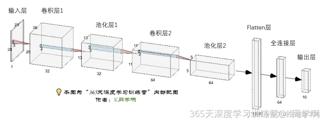
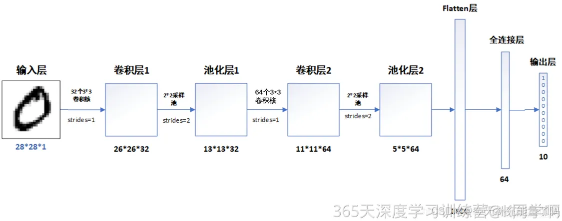
1. 构建CNN网络模型
# Define the model architecture
# 创建并设置卷积神经网络
# 卷积层:通过卷积操作对输入图像进行降维和特征抽取
# 池化层:是一种非线性形式的下采样。主要用于特征降维,压缩数据和参数的数量,减小过拟合,同时提高模型的鲁棒性。
# 全连接层:在经过几个卷积和池化层之后,神经网络中的高级推理通过全连接层来完成。
model = models.Sequential([
    # 设置二维卷积层1,设置32个3*3卷积核,activation参数将激活函数设置为ReLu函数,input_shape参数将图层的输入形状设置为(28, 28, 1)
    # ReLu函数作为激活励函数可以增强判定函数和整个神经网络的非线性特性,而本身并不会改变卷积层
    # 相比其它函数来说,ReLU函数更受青睐,这是因为它可以将神经网络的训练速度提升数倍,而并不会对模型的泛化准确度造成显著影响。
    layers.Conv2D(32, (3, 3), activation='relu', input_shape=(28, 28, 1)),
    #池化层1,2*2采样
    layers.MaxPooling2D((2, 2)),
    # 设置二维卷积层2,设置64个3*3卷积核,activation参数将激活函数设置为ReLu函数
    layers.Conv2D(64, (3, 3), activation='relu'),
    #池化层2,2*2采样
    layers.MaxPooling2D((2, 2)),

    layers.Flatten(),                    #Flatten层,连接卷积层与全连接层
    layers.Dense(64, activation='relu'), #全连接层,特征进一步提取,64为输出空间的维数,activation参数将激活函数设置为ReLu函数
    layers.Dense(10)                     #输出层,输出预期结果,10为输出空间的维数
])
# 打印网络结构
model.summary()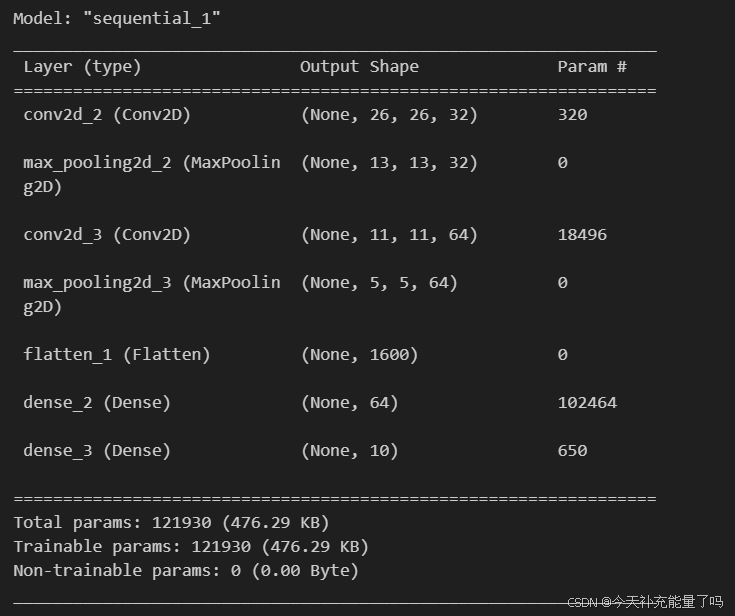
2. 编译模型
"""
这里设置优化器、损失函数以及metrics
"""
# model.compile()方法用于在配置训练方法时,告知训练时用的优化器、损失函数和准确率评测标准
model.compile(
	# 设置优化器为Adam优化器
    optimizer='adam',
	# 设置损失函数为交叉熵损失函数(tf.keras.losses.SparseCategoricalCrossentropy())
    # from_logits为True时,会将y_pred转化为概率(用softmax),否则不进行转换,通常情况下用True结果更稳定
    loss=tf.keras.losses.SparseCategoricalCrossentropy(from_logits=True),
    # 设置性能指标列表,将在模型训练时监控列表中的指标
    metrics=['accuracy'])
3. 训练模型
"""
这里设置输入训练数据集(图片及标签)、验证数据集(图片及标签)以及迭代次数epochs
关于model.fit()函数的具体介绍可参考我的博客:
https://blog.youkuaiyun.com/qq_38251616/article/details/122321757
"""
history = model.fit(
    # 输入训练集图片
	train_images,
	# 输入训练集标签
	train_labels,
	# 设置10个epoch,每一个epoch都将会把所有的数据输入模型完成一次训练。
	epochs=10,
	# 设置验证集
    validation_data=(test_images, test_labels))
Epoch 1/10
1875/1875 [==============================] - 44s 22ms/step - loss: 0.1426 - accuracy: 0.9561 - val_loss: 0.0599 - val_accuracy: 0.9797
Epoch 2/10
1875/1875 [==============================] - 69s 37ms/step - loss: 0.0456 - accuracy: 0.9859 - val_loss: 0.0385 - val_accuracy: 0.9872
Epoch 3/10
1875/1875 [==============================] - 61s 33ms/step - loss: 0.0316 - accuracy: 0.9899 - val_loss: 0.0309 - val_accuracy: 0.9906
Epoch 4/10
1875/1875 [==============================] - 44s 24ms/step - loss: 0.0237 - accuracy: 0.9921 - val_loss: 0.0302 - val_accuracy: 0.9909
Epoch 5/10
1875/1875 [==============================] - 47s 25ms/step - loss: 0.0176 - accuracy: 0.9947 - val_loss: 0.0302 - val_accuracy: 0.9910
Epoch 6/10
1875/1875 [==============================] - 55s 29ms/step - loss: 0.0141 - accuracy: 0.9954 - val_loss: 0.0310 - val_accuracy: 0.9901
Epoch 7/10
1875/1875 [==============================] - 45s 24ms/step - loss: 0.0101 - accuracy: 0.9966 - val_loss: 0.0254 - val_accuracy: 0.9931
Epoch 8/10
1875/1875 [==============================] - 36s 19ms/step - loss: 0.0094 - accuracy: 0.9971 - val_loss: 0.0369 - val_accuracy: 0.9894
Epoch 9/10
1875/1875 [==============================] - 49s 26ms/step - loss: 0.0084 - accuracy: 0.9971 - val_loss: 0.0411 - val_accuracy: 0.9897
Epoch 10/10
1875/1875 [==============================] - 50s 27ms/step - loss: 0.0072 - accuracy: 0.9976 - val_loss: 0.0344 - val_accuracy: 0.9920
三、模型预测
plt.imshow(test_images[1])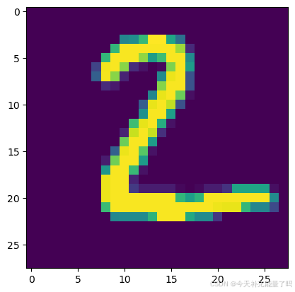
输出测试集中第一张图片的预测结果
# 输出测试集图片的预测结果
pre = model.predict(test_images) # 对所有测试图片进行预测
pre[1] # 输出第一张图片的预测结果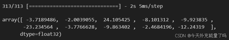


 被折叠的 条评论
为什么被折叠?
被折叠的 条评论
为什么被折叠?
 到【灌水乐园】发言


