


- 🍨 本文為🔗365天深度學習訓練營 中的學習紀錄博客
- 🍖 原作者:K同学啊 | 接輔導、項目定制
365天深度学习L2-1
一、简单线性回归
通过两个或多个变量之间的线性关系来预测结果。
二、代码实现
第1步:导入library
# Import the libraries

import numpy as np
import pandas as pd
import matplotlib.pyplot as plt
from sklearn.model_selection import train_test_split
from sklearn.linear_model import LinearRegression
第2步:读取数据
该处使用的url网络请求的数据。
# Load the data
url = "https://archive.ics.uci.edu/ml/machine-learning-databases/iris/iris.data"
names = ['花萼-length', '花萼-width', '花瓣-length', '花瓣-width', 'class']

df = pd.read_csv(url, names=names)
df.head()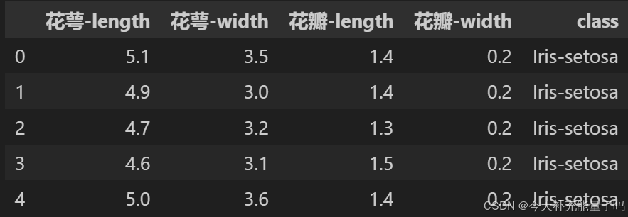
第3步:分割数据集
- 由于需要用花瓣的长度来预测花瓣的宽度,则X为第三列“花瓣-length”, y为第四列“花瓣-width”。
- 由于scikit-learn期望输入的特征数据是二维的,即
(n_samples, n_features),其中n_features是特征数, 在这种情况下,即使只有一个特征(第3列),需要显式地将其形状调整为二维。 reshape(-1, 1)的作用是将一维数组转换为二维数组,其中-1表示“自动计算行数”,1表示列数为1。最终结果是X的形状将变为(n_samples, 1)。- 这里取80%作为训练集,20%作为测试集
# Slipt the data
X = df.iloc[:, 2].values.reshape(-1, 1)
y = df.iloc[:, 3].values

X_train, X_test, y_train, y_test = train_test_split(X, y, test_size=0.2, random_state=0)
第4步:简单线性回归模型
# Linear regression model
regressor = LinearRegression()
regressor.fit(X_train, y_train)

# Predict the test set
y_pred = regressor.predict(X_test)
第5步:结果可视化
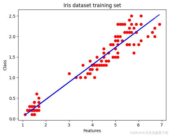
- 训练集可视化
# Visualize the training set
plt.scatter(X_train, y_train, color='red')
plt.plot(X_train, regressor.predict(X_train), color='blue')
plt.title('Iris dataset training set')
plt.xlabel('Features')
plt.ylabel('Class')
plt.show()
2. 测试集预测结果可视化
# Visualize the test set
plt.scatter(X_test, y_test, color='red')
plt.plot(X_train, regressor.predict(X_train), color='blue')
plt.title('Iris dataset test set')
plt.xlabel('Features')
plt.ylabel('Class')
plt.show()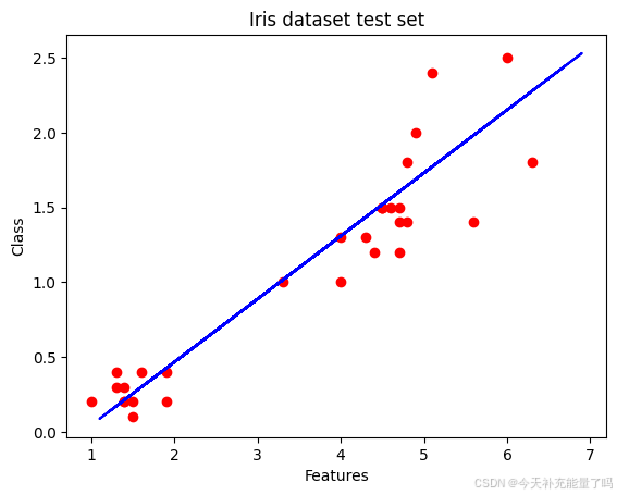


 被折叠的 条评论
为什么被折叠?
被折叠的 条评论
为什么被折叠?
 到【灌水乐园】发言


