sklearn学习——支持向量机分类

sklearn学习——支持向量机分类

1 数据集制作

小编看过很多关于支持向量机代码的博客，全是都带有自己数据集 像Iris.data，那么怎么把自己的数据给用上呢？

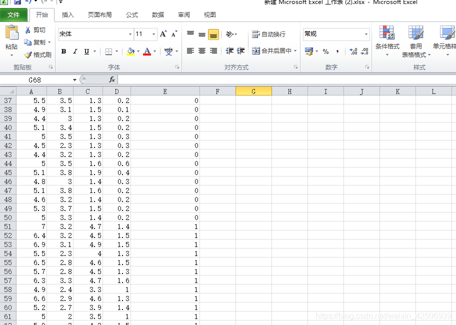
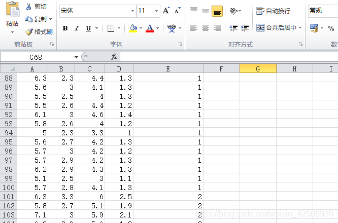
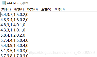
1.1 、如图，这是自己需要使用的数据集，ABCD表示数据的特征，E表示样本，分别为0，1，2三种不同的标签，现在我们的任务是通过训练支持向量机模型，从而通过已有的数据特征，来识别样本类型

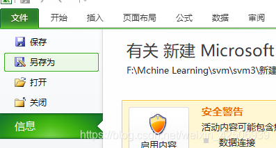
1.2、文件-另存为-选择csv文件格式

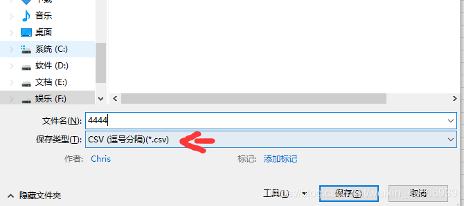
1.3 后续可以把444.csv后缀改成txt，这两种都可以使用，我下面使用的是txt，如图我制作了444.txt是训练样本，555是测试样本

2 支持向量代码

话不多说，直接代码搞起！！

2.1

from sklearn import svm
import numpy as np

# 1.读取训练数据集
path = '444.txt'
datatrain = np.loadtxt(path, dtype=float, delimiter=',')   # dtype是读出数据类型，delimiter是分隔符

# 2.读取测试数据集
path1 = '555.txt'
datatest = np.loadtxt(path1, dtype=float, delimiter=',')

# 3.划分数据与标签
x, y = np.split(datatrain, indices_or_sections=(4,), axis=1)
# x为数据，y为标签，indices_or_sections表示从4列分割
x1, y1 = np.split(datatest, indices_or_sections=(4,), axis=1)
# x为数据，y为标签，axis=1表示列分割，等于0行分割

# 3.训练svm分类器
classifier = svm.SVC(C=2, kernel='rbf', gamma='auto', decision_function_shape='ovr')
# ovr:一对多策略，ovo表示一对一
classifier.fit(x, y.ravel())     # ravel函数在降维时默认是行序优先

# 4.计算svc分类器的准确率
print("训练集：", classifier.score(x, y))
print("测试集：", classifier.score(x1, y1))

'''
# 也可直接调用accuracy_score方法计算准确率
from sklearn.metrics import accuracy_score
tra_label = classifier.predict(train_data)  # 训练集的预测标签
tes_label = classifier.predict(test_data)  # 测试集的预测标签
print("训练集：", accuracy_score(train_label, tra_label))
print("测试集：", accuracy_score(test_label, tes_label))
'''
# 查看决策函数
print('train_decision_function:\n', classifier.decision_function(x))  # 查看决策函数
# print('train_data:\n', x)                                             # 查看训练数据
# print('predict_data:\n', x1)                                          # 查看测试数据
print('predict_result:\n', classifier.predict(x1))                    # 查看测试结果
print('predict_data:\n', y1)     

代码二

如果我们的样本集中测试和训练都在一起，我们采用这个代码

from sklearn import svm
import numpy as np
from sklearn.model_selection import train_test_split

'''
define converts(字典)#
def Iris_label(s):
    it = {b'Iris-setosa': 0, b'Iris-versicolor': 1, b'Iris-virginica': 2}
    return it[s]
'''
# 1.读取数据集
path = '333.csv'
data = np.loadtxt(path, dtype=float, delimiter=',')

# 2.划分数据与标签
x, y = np.split(data, indices_or_sections=(4,), axis=1)  # x为数据，y为标签
train_data, test_data, train_label, test_label = \
    train_test_split(x, y, random_state=1, train_size=0.75,test_size=0.25)

# 3.训练svm分类器
classifier = svm.SVC(C=2, kernel='rbf', gamma='auto', decision_function_shape='ovr')
# ovr:一对多策略
classifier.fit(train_data, train_label.ravel())  # ravel函数在降维时默认是行序优先

# 4.计算svc分类器的准确率

print("训练集：", classifier.score(train_data, train_label))
print("测试集：", classifier.score(test_data, test_label))

'''
# 也可直接调用accuracy_score方法计算准确率
from sklearn.metrics import accuracy_score

tra_label = classifier.predict(train_data)  # 训练集的预测标签
tes_label = classifier.predict(test_data)  # 测试集的预测标签
print("训练集：", accuracy_score(train_label, tra_label))
print("测试集：", accuracy_score(test_label, tes_label))
'''
# 查看决策函数
print('train_decision_function:\n', classifier.decision_function(train_data))  # (90,3)
print('predict_data:\n', test_data)
print('predict_result:\n', classifier.predict(train_data))

3 代码种关键函数解释

3.1 np.loadtxt

numpy中的读取函数

numpy.loadtxt(fname, dtype=, comments=’#’, delimiter=None, converters=None, skiprows=0, usecols=None, unpack=False, ndmin=0)

fname ：读取路径
dtype ： 读取类型
comments ：这里的comment的是指, 如果行的开头为#就会跳过该行
delimiter ：分隔符
converters ：converters参数, 这个是对数据进行预处理的参数,
skiprows ：跳过第几行
unpack ：usecols=(0, 2)是指只使用0,2两列, unpack是指会把每一列当成一个向量输出, 而不是合并在一起。

3.2 np.split

split(ary, indices_or_sections, axis=1) : 把一个数组从左到右按顺序切分
参数：
ary: 要切分的数组
indices_or_sections :如果是一个整数，就用该数平均切分，如果是一个数组，为沿轴切分的位置（左开右闭）
axis： 沿着哪个维度进行切向，默认为0，横向切分。为1时，纵向切分

3.3 train_test_split

X_train,X_test, y_train, y_test =sklearn.model_selection.train_test_split(train_data,train_target,test_size=0.4, random_state=0,stratify=y_train)

train_data： 所要划分的样本特征集
train_target： 所要划分的样本结果
test_size： 样本占比，如果是整数的话就是样本的数量
random_state： 是随机数的种子。
随机数种子：其实就是该组随机数的编号，在需要重复试验的时候，保证得到一组一样的随机数。比如你每次都填1，其他参数一样的情况下你得到的随机数组是一样的。但填0或不填，每次都会不一样。
stratify 是为了保持split前类的分布。比如有100个数据，80个属于A类，20个属于B类。如果train_test_split(… test_size=0.25, stratify = y_all), 那么split之后数据如下：
training: 75个数据，其中60个属于A类，15个属于B类。
testing: 25个数据，其中20个属于A类，5个属于B类

3.4 svm.SVC

sklearn.svm.SVC(C=1.0, kernel=‘rbf’, degree=3, gamma=‘auto’, coef0=0.0, shrinking=True, probability=False,
tol=0.001, cache_size=200, class_weight=None, verbose=False, max_iter=-1, decision_function_shape=None,random_state=None)

参数：
C：C-SVC的惩罚参数C?默认值是1.0
C越大，相当于惩罚松弛变量，希望松弛变量接近0，即对误分类的惩罚增大，趋向于对训练集全分对的情况，这样对训练集测试时准确率很高，但泛化能力弱。C值小，对误分类的惩罚减小，允许容错，将他们当成噪声点，泛化能力较强。

kernel ：核函数，默认是rbf，可以是‘linear’, ‘poly’, ‘rbf’, ‘sigmoid’, ‘precomputed’
　　0 – 线性：u’v
　　 1 – 多项式：(gamma*u’v + coef0)^degree
　　2 – RBF函数：exp(-gamma|u-v|^2)
　　3 –sigmoid：tanh(gammau’*v + coef0)

degree ：多项式poly函数的维度，默认是3，选择其他核函数时会被忽略。
gamma ： ‘rbf’,‘poly’ 和‘sigmoid’的核函数参数。默认是’auto’，则会选择1/n_features
coef0 ：核函数的常数项。对于‘poly’和 ‘sigmoid’有用。
probability ：是否采用概率估计？.默认为False
shrinking ：是否采用shrinking heuristic方法，默认为true
tol ：停止训练的误差值大小，默认为1e-3
cache_size ：核函数cache缓存大小，默认为200
class_weight ：类别的权重，字典形式传递。设置第几类的参数C为weight*C(C-SVC中的C)
verbose ：允许冗余输出？
max_iter ：最大迭代次数。-1为无限制。
decision_function_shape ：‘ovo’, ‘ovr’ or None, default=None3
random_state ：数据洗牌时的种子值，int值

主要调节的参数有：C、kernel、degree、gamma、coef0、decision_function_shape。