


注:本文为 “Big O notation ” 相关合辑。
英文引文,机翻未校。
中文引文,略排未校。
如有内容异常,请看原文。
Big O notation
大 O 符号
Big O notation (with a capital letter O, not a zero), also called Landau’s symbol, is a symbolism used in complexity theory, computer science, and mathematics to describe the asymptotic behavior of functions. Basically, it tells you how fast a function grows or declines.
大 O 符号(字母 O 为大写,非数字 0),又称朗道符号(Landau’s symbol),是复杂度理论、计算机科学与数学领域中用于描述函数渐近行为的一种符号体系。本质上,它能表明函数增长或衰减的速率。
Landau’s symbol comes from the name of the German number theoretician Edmund Landau who invented the notation. The letter O is used because the rate of growth of a function is also called its order.
朗道符号的名称源自该符号的发明者 —— 德国数论学家埃德蒙・朗道(Edmund Landau)。选用字母 O 是因为函数的增长速率也被称为函数的 “阶”(order)。
For example, when analyzing some algorithm, one might find that the time (or the number of steps) it takes to complete a problem of size
n
n
n is given by
T
(
n
)
=
4
n
2
−
2
n
+
2
T (n) = 4n^2 - 2n + 2
T(n)=4n2−2n+2. If we ignore constants (which makes sense because those depend on the particular hardware the program is run on) and slower growing terms, we could say “
T
(
n
)
T (n)
T(n) grows at the order of
n
2
n^2
n2” and write:
T
(
n
)
=
O
(
n
2
)
T (n) = O (n^2)
T(n)=O(n2).
例如,在分析某一算法时,可能会发现解决规模为
n
n
n 的问题所需的时间(或步骤数)可表示为
T
(
n
)
=
4
n
2
−
2
n
+
2
T (n) = 4n^2 - 2n + 2
T(n)=4n2−2n+2。若忽略常数项(忽略常数项是合理的,因为常数项取决于程序运行所依赖的特定硬件)和增长较慢的项,我们可以认为 “
T
(
n
)
T (n)
T(n) 以
n
2
n^2
n2 的阶增长”,并记为:
T
(
n
)
=
O
(
n
2
)
T (n) = O (n^2)
T(n)=O(n2)。
In mathematics, it is often important to get a handle on the error term of an approximation. For instance, people will write
在数学中,掌握近似计算的误差项通常十分重要。例如,人们会写下
e
x
=
1
+
x
+
x
2
2
+
O
(
x
3
)
for
x
→
0
e^x = 1 + x + \frac {x^2}{2} + O (x^3) \quad \text {for } x \to 0
ex=1+x+2x2+O(x3)for x→0
to express the fact that the error is smaller in absolute value than some constant times
x
3
x^3
x3 if
x
x
x is close enough to 0.
该式表示:当
x
x
x 足够接近 0 时,上述近似的误差绝对值小于某个常数与
x
3
x^3
x3 的乘积。
For the formal definition, suppose
f
(
x
)
f (x)
f(x) and
g
(
x
)
g (x)
g(x) are two functions defined on some subset of the real numbers. We write
其形式化定义如下:设
f
(
x
)
f (x)
f(x) 和
g
(
x
)
g (x)
g(x) 是定义在实数集某一子集上的两个函数。我们记
f
(
x
)
=
O
(
g
(
x
)
)
f (x) = O (g (x))
f(x)=O(g(x))
(or
f
(
x
)
=
O
(
g
(
x
)
)
f (x) = O (g (x))
f(x)=O(g(x)) for
x
→
∞
x \to \infty
x→∞ to be more precise) if and only if there exist constants
N
N
N and
C
C
C such that
∣
f
(
x
)
∣
≤
C
∣
g
(
x
)
∣
for all
x
>
N
.
|f (x)| \leq C|g (x)| \quad \text {for all } x > N.
∣f(x)∣≤C∣g(x)∣for all x>N.
(为更精确,也可记为当
x
→
∞
x \to \infty
x→∞ 时,
f
(
x
)
=
O
(
g
(
x
)
)
f (x) = O (g (x))
f(x)=O(g(x))),当且仅当存在常数
N
N
N 和
C
C
C,使得对所有满足
x
>
N
x > N
x>N 的
x
x
x,均有
∣
f
(
x
)
∣
≤
C
∣
g
(
x
)
∣
.
|f (x)| \leq C|g (x)|.
∣f(x)∣≤C∣g(x)∣.
Intuitively, this means that
f
f
f does not grow faster than
g
g
g.
从直观上理解,该定义表明
f
f
f 的增长速率不超过
g
g
g。
If
a
a
a is some real number, we write
若
a
a
a 为某一实数,我们记
f
(
x
)
=
O
(
g
(
x
)
)
for
x
>
a
f (x) = O (g (x)) \quad \text {for } x > a
f(x)=O(g(x))for x>a
if and only if there exist constants
d
>
0
d > 0
d>0 and
C
C
C such that
∣
f
(
x
)
∣
≤
C
∣
g
(
x
)
∣
for all
x
with
∣
x
−
a
∣
<
d
.
|f (x)| \leq C|g (x)| \quad \text {for all } x \text { with } |x - a| < d.
∣f(x)∣≤C∣g(x)∣for all x with ∣x−a∣<d.
当且仅当存在常数
d
>
0
d > 0
d>0 和
C
C
C,使得对所有满足
∣
x
−
a
∣
<
d
|x - a| < d
∣x−a∣<d 的
x
x
x,均有
∣
f
(
x
)
∣
≤
C
∣
g
(
x
)
∣
|f (x)| \leq C|g (x)|
∣f(x)∣≤C∣g(x)∣。
The first definition is the only one used in computer science (where typically only positive functions with a natural number
n
n
n as argument are considered; the absolute values can then be ignored), while both usages appear in mathematics.
计算机科学领域仅使用上述第一个定义(该领域通常只考虑以自然数
n
n
n 为自变量的正函数,因此绝对值符号可省略),而数学领域则会同时使用上述两种定义。
Here is a list of classes of functions that are commonly encountered when analyzing algorithms. The slower growing functions are listed first.
c
c
c is some arbitrary constant.
下表列出了算法分析中常见的函数类别,按函数增长速率由慢到快排序。其中
c
c
c 为任意常数。
算法复杂度符号
| O ( 1 ) O (1) O(1) | constant 常数阶 |
|---|---|
| O ( log ( n ) ) O (\log (n)) O(log(n)) | logarithmic 对数阶 |
| O ( ( log ( n ) ) c ) O ((\log (n))^c) O((log(n))c) | polylogarithmic 多项式对数阶 |
| O ( n ) O (n) O(n) | linear 线性阶 |
| O ( n 2 ) O (n^2) O(n2) | quadratic 平方阶 |
| O ( n c ) O (n^c) O(nc) | polynomial 多项式阶 |
| O ( c n ) O (c^n) O(cn) | exponential 指数阶 |
Note that
O
(
n
c
)
O (n^c)
O(nc) and
O
(
c
n
)
O (c^n)
O(cn) are very different. The latter grows much, much faster, no matter how big the constant
c
c
c is. A function that grows faster than any power of
n
n
n is called superpolynomial. One that grows slower than an exponential function of the form
c
n
c^n
cn is called subexponential. An algorithm can require time that is both superpolynomial and subexponential; examples of this include the fastest algorithms known for integer factorization.
需注意,
O
(
n
c
)
O (n^c)
O(nc) 与
O
(
c
n
)
O (c^n)
O(cn) 存在显著差异。无论常数
c
c
c 取值多大,后者的增长速率都远快于前者。增长速率超过
n
n
n 的任意次幂的函数称为 “超多项式函数”(superpolynomial);增长速率慢于
c
n
c^n
cn 形式指数函数的函数称为 “亚指数函数”(subexponential)。有些算法的时间复杂度既属于超多项式级,又属于亚指数级,例如目前已知的最快整数分解算法。
Note, too, that
O
(
l
o
g
n
)
O (log\ n)
O(log n) is exactly the same as
O
(
l
o
g
(
n
c
)
)
O (log (n^c))
O(log(nc)). The logarithms differ only by a constant factor, and the big O notation ignores that. Similarly, logs with different constant bases are equivalent.
另需注意,
O
(
l
o
g
n
)
O (log\ n)
O(log n) 与
O
(
l
o
g
(
n
c
)
)
O (log (n^c))
O(log(nc)) 完全等价。这是因为这两个对数表达式仅相差一个常数因子,而大 O 符号会忽略常数因子。同理,以不同常数为底的对数函数在大 O 符号下也是等价的。
The above list is useful because of the following fact: if a function
f
(
n
)
f (n)
f(n) is a sum of functions, one of which grows faster than the others, then the faster growing one determines the order of
f
(
n
)
f (n)
f(n).
上述函数类别列表之所以实用,是因为存在以下规律:若函数
f
(
n
)
f (n)
f(n) 是多个函数的和,且其中一个函数的增长速率快于其他所有函数,则该增长最快的函数决定了
f
(
n
)
f (n)
f(n) 的阶。
Example: If
示例:若
f
(
n
)
=
10
l
o
g
(
n
)
+
5
(
l
o
g
(
n
)
)
3
+
7
n
+
3
n
2
+
6
n
3
f (n) = 10log (n) + 5 (log (n))^3 + 7n + 3n^2 + 6n^3
f(n)=10log(n)+5(log(n))3+7n+3n2+6n3, then
f
(
n
)
=
O
(
n
3
)
f (n) = O (n^3)
f(n)=O(n3).
One caveat here: the number of summands has to be constant and may not depend on
n
n
n. This notation can also be used with multiple variables and with other expressions on the right side of the equal sign. The notation:
此处需注意一点:求和项的数量必须是常数,且不得依赖于
n
n
n。大 O 符号也可用于多变量场景,且等号右侧可出现其他表达式。例如符号:
f
(
n
,
m
)
=
n
2
+
m
3
+
O
(
n
+
m
)
f (n, m) = n^2 + m^3 + O (n + m)
f(n,m)=n2+m3+O(n+m)
represents the statement:
表示如下含义:
∃
C
∃
N
∀
n
,
m
>
N
:
f
(
n
,
m
)
≤
n
2
+
m
3
+
C
(
n
+
m
)
\exists C \exists N \forall n, m > N: f (n, m) \leq n^2 + m^3 + C (n + m)
∃C∃N∀n,m>N:f(n,m)≤n2+m3+C(n+m)
(存在常数
C
C
C 和
N
N
N,使得对所有满足
n
,
m
>
N
n, m > N
n,m>N 的
n
n
n 和
m
m
m,均有
f
(
n
,
m
)
≤
n
2
+
m
3
+
C
(
n
+
m
)
f (n, m) \leq n^2 + m^3 + C (n + m)
f(n,m)≤n2+m3+C(n+m))
Obviously, this notation is abusing the equality symbol, since it violates the axiom of equality: “things equal to the same thing are equal to each other”. To be more formally correct, some people (mostly mathematicians, as opposed to computer scientists) prefer to define
O
(
g
(
x
)
)
O (g (x))
O(g(x)) as a set-valued function, whose value is all functions that do not grow faster than
g
(
x
)
g (x)
g(x), and use set membership notation to indicate that a specific function is a member of the set thus defined. Both forms are in common use, but the sloppier equality notation is more common at present.
显然,这种符号表示方式对等号的使用并不严谨,因为它违背了等式公理:“与同一事物相等的事物彼此相等”。为了在形式上更严谨,部分学者(以数学家为主,计算机科学家较少)更倾向于将
O
(
g
(
x
)
)
O (g (x))
O(g(x)) 定义为一个集值函数,其取值为所有增长速率不超过
g
(
x
)
g (x)
g(x) 的函数构成的集合,并使用集合隶属符号(
∈
\in
∈)表示某一特定函数属于该集合。这两种表示形式均被广泛使用,但目前不那么严谨的等号表示法更为常见。
Another point of sloppiness is that the parameter whose asymptotic behaviour is being examined is not clear. A statement such as
f
(
x
,
y
)
=
O
(
g
(
x
,
y
)
)
f (x, y) = O (g (x, y))
f(x,y)=O(g(x,y)) requires some additional explanation to make clear what is meant. Still, this problem is rare in practice.
另一个不严谨之处在于,有时未明确指出所分析渐近行为对应的参数。例如,对于
f
(
x
,
y
)
=
O
(
g
(
x
,
y
)
)
f (x, y) = O (g (x, y))
f(x,y)=O(g(x,y)) 这样的表述,需要额外说明其具体含义(即针对哪个参数的渐近行为)。不过,在实际应用中,这类问题很少出现。
Related notations
相关符号
In addition to the big O notation, another Landau symbol is used in mathematics: the little o. Informally,
f
(
x
)
=
o
(
g
(
x
)
)
f (x) = o (g (x))
f(x)=o(g(x)) means that
f
f
f grows much slower than
g
g
g and is insignificant in comparison.
除大 O 符号外,数学领域还会使用另一种朗道符号:小 o 符号(little o)。从直观上看,
f
(
x
)
=
o
(
g
(
x
)
)
f (x) = o (g (x))
f(x)=o(g(x)) 表示
f
f
f 的增长速率远慢于
g
g
g,因此在与
g
g
g 的比较中,
f
f
f 可视为无关紧要的项。
Formally, we write
f
(
x
)
=
o
(
g
(
x
)
)
f (x) = o (g (x))
f(x)=o(g(x)) (for
x
→
∞
x \to \infty
x→∞) if and only if for every
C
>
0
C > 0
C>0 there exists a real number
N
N
N such that for all
x
>
N
x > N
x>N we have
∣
f
(
x
)
∣
<
C
∣
g
(
x
)
∣
|f (x)| < C|g (x)|
∣f(x)∣<C∣g(x)∣; if
g
(
x
)
≠
0
g (x) \neq 0
g(x)=0, this is equivalent to
lim
x
→
∞
f
(
x
)
g
(
x
)
=
0
\lim_{x \to \infty} \frac {f (x)}{g (x)} = 0
limx→∞g(x)f(x)=0.
其形式化定义为:我们记
f
(
x
)
=
o
(
g
(
x
)
)
f (x) = o (g (x))
f(x)=o(g(x))(当
x
→
∞
x \to \infty
x→∞ 时),当且仅当对任意
C
>
0
C > 0
C>0,存在实数
N
N
N,使得对所有满足
x
>
N
x > N
x>N 的
x
x
x,均有
∣
f
(
x
)
∣
<
C
∣
g
(
x
)
∣
|f (x)| < C|g (x)|
∣f(x)∣<C∣g(x)∣;若
g
(
x
)
≠
0
g (x) \neq 0
g(x)=0,则该定义等价于
lim
x
→
∞
f
(
x
)
g
(
x
)
=
0
\lim_{x \to \infty} \frac {f (x)}{g (x)} = 0
limx→∞g(x)f(x)=0。
Also, if
a
a
a is some real number, we write
f
(
x
)
=
o
(
g
(
x
)
)
f (x) = o (g (x))
f(x)=o(g(x)) for
x
→
a
x \to a
x→a if and only if for every
C
>
0
C > 0
C>0 there exists a positive real number
d
d
d such that for all
x
x
x with
∣
x
−
a
∣
<
d
|x - a| < d
∣x−a∣<d we have
∣
f
(
x
)
∣
<
C
∣
g
(
x
)
∣
|f (x)| < C|g (x)|
∣f(x)∣<C∣g(x)∣; if
g
(
x
)
≠
0
g (x) \neq 0
g(x)=0, this is equivalent to
lim
x
→
a
f
(
x
)
g
(
x
)
=
0
\lim_{x \to a} \frac {f (x)}{g (x)} = 0
limx→ag(x)f(x)=0.
此外,若
a
a
a 为某一实数,我们记
f
(
x
)
=
o
(
g
(
x
)
)
f (x) = o (g (x))
f(x)=o(g(x))(当
x
→
a
x \to a
x→a 时),当且仅当对任意
C
>
0
C > 0
C>0,存在正实数
d
d
d,使得对所有满足
∣
x
−
a
∣
<
d
|x - a| < d
∣x−a∣<d 的
x
x
x,均有
∣
f
(
x
)
∣
<
C
∣
g
(
x
)
∣
|f (x)| < C|g (x)|
∣f(x)∣<C∣g(x)∣;若
g
(
x
)
≠
0
g (x) \neq 0
g(x)=0,则该定义等价于
lim
x
→
a
f
(
x
)
g
(
x
)
=
0
\lim_{x \to a} \frac {f (x)}{g (x)} = 0
limx→ag(x)f(x)=0。
Big O is the most commonly-used of five notations for comparing functions:
在用于比较函数的五种符号中,大 O 符号的使用最为广泛:
| Notation | Definition | Analogy |
|---|---|---|
| f ( n ) = O ( g ( n ) ) f (n) = O (g (n)) f(n)=O(g(n)) | see above |
≤
\leq
≤ 不超过 |
| f ( n ) = o ( g ( n ) ) f (n) = o (g (n)) f(n)=o(g(n)) | see above |
≪
\ll
≪ 远小于 |
| f ( n ) = Ω ( g ( n ) ) f (n) = \Omega (g (n)) f(n)=Ω(g(n)) | g ( n ) = O ( f ( n ) ) g (n) = O (f (n)) g(n)=O(f(n)) |
≥
\geq
≥ 不小于 |
| f ( n ) = ω ( g ( n ) ) f (n) = \omega (g (n)) f(n)=ω(g(n)) | g ( n ) = o ( f ( n ) ) g (n) = o (f (n)) g(n)=o(f(n)) |
≫
\gg
≫ 远大于 |
| f ( n ) = Θ ( g ( n ) ) f (n) = \Theta (g (n)) f(n)=Θ(g(n)) | f ( n ) = O ( g ( n ) ) f (n) = O (g (n)) f(n)=O(g(n)) and g ( n ) = O ( f ( n ) ) g (n) = O (f (n)) g(n)=O(f(n)) |
=
=
= 等价 |
The notations
Ω
\Omega
Ω and
Θ
\Theta
Θ are often used in computer science; the lowercase
o
o
o is common in mathematics but rare in computer science. The lowercase
ω
\omega
ω is rarely used.
Ω
\Omega
Ω 和
Θ
\Theta
Θ 符号在计算机科学中经常使用;小写的
o
o
o 符号在数学中较为常见,但在计算机科学中很少使用;小写的
ω
\omega
ω 符号则极少使用。
A common error is to confuse these by using
O
O
O when
Θ
\Theta
Θ is meant. For example, one might say “heapsort is
O
(
n
l
o
g
n
)
O (n log n)
O(nlogn)” when the intended meaning was “heapsort is
Θ
(
n
l
o
g
n
)
\Theta (n log n)
Θ(nlogn)”. Both statements are true, but the latter is a stronger claim.
一个常见错误是混淆这些符号的含义,例如本应使用
Θ
\Theta
Θ 却使用了
O
O
O。例如,有人可能会说 “堆排序(heapsort)的时间复杂度是
O
(
n
l
o
g
n
)
O (n log n)
O(nlogn)”,但实际想表达的是 “堆排序的时间复杂度是
Θ
(
n
l
o
g
n
)
\Theta (n log n)
Θ(nlogn)”。这两种表述均正确,但后者的断言更强(前者仅表示上界,后者表示上界与下界一致,即精确阶)。
The notations described here are very useful. They are used for approximating formulas for analysis of algorithms, and for the definitions of terms in complexity theory (e.g. polynomial time).
本文介绍的这些符号具有重要用途,它们可用于算法分析中的公式近似,也可用于复杂度理论中相关术语的定义(例如 “多项式时间”)。
Understanding Big O
理解大 O 符号
Introduction
引言
How efficient is an algorithm or piece of code? Efficiency covers lots of resources, including:
一个算法或一段代码的效率如何?效率涉及多种资源,包括:
-
CPU (time) usage
CPU(时间)使用率 -
memory usage
内存使用率 -
disk usage
磁盘使用率 -
network usage
网络使用率
All are important but we will mostly talk about time complexity (CPU usage).
这些资源都很重要,但本文将主要讨论时间复杂度(即 CPU 使用率)。
Be careful to differentiate between:
需注意区分以下两个概念:
-
Performance: how much time/memory/disk/… is actually used when a program is run. This depends on the machine, compiler, etc. as well as the code.
性能(Performance):程序运行时实际消耗的时间、内存、磁盘空间等资源的量。性能不仅取决于代码,还与运行环境(如机器、编译器等)相关。 -
Complexity: how do the resource requirements of a program or algorithm scale, i.e., what happens as the size of the problem being solved gets larger?
复杂度(Complexity):程序或算法的资源需求如何随问题规模变化,即当待解决问题的规模增大时,资源需求会发生怎样的变化?
Complexity affects performance but not the other way around.
复杂度会影响性能,但性能不会反过来影响复杂度。
The time required by a function/procedure is proportional to the number of “basic operations” that it performs. Here are some examples of basic operations:
一个函数 / 过程所需的时间与其执行的 “基本操作” 数量成正比。以下是基本操作的一些示例:
-
one arithmetic operation (e.g., +, )
一次算术运算(如 +、) -
one assignment (e.g. x := 0)
一次赋值操作(如 x := 0) -
one test (e.g., x = 0 x = 0 x=0)
一次判断操作(如 x = 0 x = 0 x=0) -
one read (of a primitive type: integer, float, character, boolean)
一次读取操作(读取基本数据类型:整数、浮点数、字符、布尔值) -
one write (of a primitive type: integer, float, character, boolean)
一次写入操作(写入基本数据类型:整数、浮点数、字符、布尔值)
Some functions/procedures perform the same number of operations every time they are called. For example, StackSize in the Stack implementation always returns the number of elements currently in the stack or states that the stack is empty, then we say that StackSize takes constant time.
有些函数 / 过程每次被调用时执行的操作数量都是固定的。例如,栈(Stack)实现中的 StackSize 函数,其功能是返回栈中当前的元素数量或提示栈为空,这类函数的时间复杂度被称为 “常数时间”。
Other functions/procedures may perform different numbers of operations, depending on the value of a parameter. For example, in the BubbleSort algorithm, the number of elements in the array determines the number of operations performed by the algorithm. This parameter (number of elements) is called the problem size/input size.
另一些函数 / 过程执行的操作数量则会随参数值变化。例如,在冒泡排序(BubbleSort)算法中,数组的元素数量决定了算法执行的操作数量。这个参数(元素数量)被称为 “问题规模 / 输入规模”。
When we are trying to find the complexity of the function/procedure/algorithm/program, we are not interested in the exact number of operations that are being performed. Instead, we are interested in the relation of the number of operations to the problem size.
在分析函数、过程、算法或程序的复杂度时,我们并不关注其执行的精确操作数量,而是关注操作数量与问题规模之间的关系。
Typically, we are usually interested in the worst case: what is the maximum number of operations that might be performed for a given problem size. For example, inserting an element into an array, we have to move the current element and all of the elements that come after it one place to the right in the array. In the worst case, inserting at the beginning of the array, all of the elements in the array must be moved. Therefore, in the worst case, the time for insertion is proportional to the number of elements in the array, and we say that the worst-case time for the insertion operation is linear in the number of elements in the array. For a linear-time algorithm, if the problem size doubles, the number of operations also doubles.
通常,我们最关注 “最坏情况”:对于给定的问题规模,算法可能执行的最大操作数量是多少。例如,向数组中插入一个元素时,需要将当前位置及后续所有元素向右移动一位。在最坏情况下(即从数组开头插入元素),数组中的所有元素都需要移动。因此,最坏情况下,插入操作的时间与数组元素数量成正比,我们称插入操作的最坏情况时间复杂度为 “与数组元素数量呈线性关系”。对于线性时间算法,若问题规模翻倍,其执行的操作数量也会翻倍。
Big-O notation
大 O 符号
We express complexity using big-O notation.
我们使用大 O 符号来表示复杂度。
For a problem of size
N
N
N:
对于规模为
N
N
N 的问题:
-
a constant-time algorithm is “order 1”: O ( 1 ) O (1) O(1)
常数时间算法的复杂度为 “1 阶”: O ( 1 ) O (1) O(1) -
a linear-time algorithm is “order N N N”: O ( N ) O (N) O(N)
线性时间算法的复杂度为 “ N N N 阶”: O ( N ) O (N) O(N) -
a quadratic-time algorithm is “order N N N squared”: O ( N 2 ) O (N^2) O(N2)
平方时间算法的复杂度为 “ N N N 平方阶”: O ( N 2 ) O (N^2) O(N2)
Note that the big-O expressions do not have constants or low-order terms. This is because, when
N
N
N gets large enough, constants and low-order terms don’t matter (a constant-time algorithm will be faster than a linear-time algorithm, which will be faster than a quadratic-time algorithm).
需注意,大 O 表达式中不包含常数项和低阶项。这是因为当
N
N
N 足够大时,常数项和低阶项对复杂度的影响可忽略不计(常数时间算法始终快于线性时间算法,而线性时间算法始终快于平方时间算法)。
Formal definition:
形式化定义:
A function
T
(
N
)
T (N)
T(N) is
O
(
F
(
N
)
)
O (F (N))
O(F(N)) if for some constant
c
c
c and for values of
N
N
N greater than some value
n
0
n_0
n0
若存在常数
c
c
c 和
n
0
n_0
n0,使得当
N
>
n
0
N > n_0
N>n0 时,有
T
(
N
)
≤
c
×
F
(
N
)
T (N) \leq c \times F (N)
T(N)≤c×F(N)
则称函数
T
(
N
)
T (N)
T(N) 是
O
(
F
(
N
)
)
O (F (N))
O(F(N)) 的。
The idea is that
T
(
N
)
T (N)
T(N) is the exact complexity of a procedure/function/algorithm as a function of the problem size
N
N
N, and that
F
(
N
)
F (N)
F(N) is an upper-bound on that complexity (i.e., the actual time/space or whatever for a problem of size
N
N
N will be no worse than
F
(
N
)
F (N)
F(N)).
该定义的核心思想是:
T
(
N
)
T (N)
T(N) 是过程 / 函数 / 算法的精确复杂度(以问题规模
N
N
N 为自变量),而
F
(
N
)
F (N)
F(N) 是该复杂度的一个上界(即对于规模为
N
N
N 的问题,实际消耗的时间、空间等资源不会超过
F
(
N
)
F (N)
F(N) 所描述的水平)。
In practice, we want the smallest
F
(
N
)
F (N)
F(N) – the least upper bound on the actual complexity. For example, consider:
在实际应用中,我们希望找到最小的
F
(
N
)
F (N)
F(N)(即实际复杂度的 “最小上界”)。例如,考虑以下精确复杂度函数:
T
(
N
)
=
3
×
N
2
+
5
T (N) = 3 \times N^2 + 5
T(N)=3×N2+5
We can show that
T
(
N
)
T (N)
T(N) is
O
(
N
2
)
O (N^2)
O(N2) by choosing
c
=
4
c = 4
c=4 and
n
0
=
2
n_0 = 2
n0=2.
This is because for all values of
N
N
N greater than 2:
通过选择
c
=
4
c = 4
c=4 和
n
0
=
2
n_0 = 2
n0=2,可证明
T
(
N
)
=
O
(
N
2
)
T (N) = O (N^2)
T(N)=O(N2)。
这是因为当
N
>
2
N > 2
N>2 时,总有:
3
×
N
2
+
5
≤
4
×
N
2
3 \times N^2 + 5 \leq 4 \times N^2
3×N2+5≤4×N2
T
(
N
)
T (N)
T(N) is not
O
(
N
)
O (N)
O(N), because whatever constant
c
c
c and value
n
0
n_0
n0 you choose, there is always a value of
N
>
n
0
N > n_0
N>n0 such that
(
3
×
N
2
+
5
)
>
(
c
×
N
)
(3 \times N^2 + 5) > (c \times N)
(3×N2+5)>(c×N).
T
(
N
)
T (N)
T(N) 不属于
O
(
N
)
O (N)
O(N),因为无论选择何种常数
c
c
c 和
n
0
n_0
n0,总能找到满足
N
>
n
0
N > n_0
N>n0 的
N
N
N,使得
(
3
×
N
2
+
5
)
>
(
c
×
N
)
(3 \times N^2 + 5) > (c \times N)
(3×N2+5)>(c×N)。
How to Determine Complexities
如何确定复杂度
In general, how can you determine the running time of a piece of code? The answer is that it depends on what kinds of statements are used.
通常情况下,如何确定一段代码的运行时间?答案是:运行时间取决于代码中使用的语句类型。
Sequence of statements
顺序语句
statement 1;
statement 2;
...
statement k;
The total time is found by adding the times for all statements:
顺序语句的总运行时间为所有语句运行时间之和:
total time = time (statement 1) + time (statement 2) + … + time (statement k)
总时间 = 语句 1 的时间 + 语句 2 的时间 + … + 语句 k 的时间
If each statement is “simple” (only involves basic operations) then the time for each statement is constant and the total time is also constant:
O
(
1
)
O (1)
O(1).
若每个语句都是 “简单语句”(仅包含基本操作),则每个语句的运行时间均为常数,因此总运行时间也为常数:
O
(
1
)
O (1)
O(1)。
If-Then-Else
条件语句(If-Then-Else)
if (cond) then
block 1 (sequence of statements)
else
block 2 (sequence of statements)
end if;
Here, either block 1 will execute, or block 2 will execute. Therefore, the worst-case time is the slower of the two possibilities:
在条件语句中,要么执行代码块 1(block 1),要么执行代码块 2(block 2)。因此,最坏情况时间复杂度为两个代码块中运行时间较长的那个:
max (time (block 1), time (block 2))
max (代码块 1 的时间,代码块 2 的时间)
If block 1 takes
O
(
1
)
O (1)
O(1) and block 2 takes
O
(
N
)
O (N)
O(N), the if-then-else statement would be
O
(
N
)
O (N)
O(N).
若代码块 1 的时间复杂度为
O
(
1
)
O (1)
O(1),代码块 2 的时间复杂度为
O
(
N
)
O (N)
O(N),则该条件语句的时间复杂度为
O
(
N
)
O (N)
O(N)。
Loops
循环语句
for I in 1 .. N loop
sequence of statements
end loop;
The loop executes
N
N
N times, so the sequence of statements also executes
N
N
N times. If we assume the statements are
O
(
1
)
O (1)
O(1), the total time for the for loop is
N
×
O
(
1
)
N \times O (1)
N×O(1), which is
O
(
N
)
O (N)
O(N) overall.
该循环执行
N
N
N 次,因此循环内部的语句序列也执行
N
N
N 次。若假设循环内部语句的时间复杂度为
O
(
1
)
O (1)
O(1),则该 for 循环的总时间复杂度为
N
×
O
(
1
)
N \times O (1)
N×O(1),即整体为
O
(
N
)
O (N)
O(N)。
Nested loops
嵌套循环
for I in 1 .. N loop
for J in 1 .. M loop
sequence of statements
end loop;
end loop;
The outer loop executes
N
N
N times. Every time the outer loop executes, the inner loop executes
M
M
M times. As a result, the statements in the inner loop execute a total of
N
×
M
N \times M
N×M times. Thus, the complexity is
O
(
N
×
M
)
O (N \times M)
O(N×M).
外层循环执行
N
N
N 次,每次外层循环执行时,内层循环都会执行
M
M
M 次。因此,内层循环中的语句总共执行
N
×
M
N \times M
N×M 次,该嵌套循环的时间复杂度为
O
(
N
×
M
)
O (N \times M)
O(N×M)。
In a common special case where the stopping condition of the inner loop is
J
<
N
J < N
J<N instead of
J
<
M
J < M
J<M (i.e., the inner loop also executes
N
N
N times), the total complexity for the two loops is
O
(
N
2
)
O (N^2)
O(N2).
在一种常见的特殊情况下,若内层循环的终止条件为
J
<
N
J < N
J<N(而非
J
<
M
J < M
J<M),即内层循环也执行
N
N
N 次,则该嵌套循环的总时间复杂度为
O
(
N
2
)
O (N^2)
O(N2)。
Statements with function/procedure calls
包含函数 / 过程调用的语句
When a statement involves a function/procedure call, the complexity of the statement includes the complexity of the function/procedure. Assume that you know that function/procedure
f
f
f takes constant time, and that function/procedure
g
g
g takes time proportional to (linear in) the value of its parameter
k
k
k. Then the statements below have the time complexities indicated:
当语句中包含函数 / 过程调用时,该语句的复杂度需包含被调用函数 / 过程的复杂度。假设已知函数 / 过程
f
f
f 的时间复杂度为常数,函数 / 过程
g
g
g 的时间复杂度与参数
k
k
k 成正比(即线性关系),则以下语句的时间复杂度如下:
-
f ( k ) f (k) f(k) has O ( 1 ) O (1) O(1)
f ( k ) f (k) f(k) 的时间复杂度为 O ( 1 ) O (1) O(1) -
g ( k ) g (k) g(k) has O ( k ) O (k) O(k)
g ( k ) g (k) g(k) 的时间复杂度为 O ( k ) O (k) O(k)
When a loop is involved, the same rule applies. For example:
当循环中包含函数 / 过程调用时,上述规则同样适用。例如,以下代码:
for J in 1 .. N loop
g (J);
end loop;
has complexity
O
(
N
2
)
O (N^2)
O(N2). The loop executes
N
N
N times and each function/procedure call
g
(
J
)
g (J)
g(J) is complexity
O
(
J
)
O (J)
O(J) (and since
J
≤
N
J \leq N
J≤N,
O
(
J
)
≤
O
(
N
)
O (J) \leq O (N)
O(J)≤O(N)).
的时间复杂度为
O
(
N
2
)
O (N^2)
O(N2)。该循环执行
N
N
N 次,每次调用函数
g
(
J
)
g (J)
g(J) 的时间复杂度为
O
(
J
)
O (J)
O(J)(由于
J
≤
N
J \leq N
J≤N,故
O
(
J
)
≤
O
(
N
)
O (J) \leq O (N)
O(J)≤O(N)),因此总复杂度为
N
×
O
(
N
)
=
O
(
N
2
)
N \times O (N) = O (N^2)
N×O(N)=O(N2)。
大 O 符号
ref: wikipedia.
大 O 符号(英语:Big O notation),又称为渐近符号,是用于描述函数渐近行为的数学符号。更确切地说,它是用另一个(通常更简单的)函数来描述一个函数数量级的渐近上界。在数学中,它一般用来刻画被截断的无穷级数尤其是渐近级数的剩余项;在计算机科学中,它在分析算法复杂性的方面非常有用。
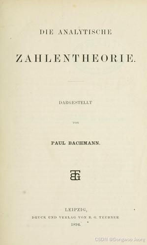
大 O 符号是由德国数论学家保罗·巴赫曼在其 1892 年的著作《解析数论》(Analytische Zahlentheorie)中首先引入的。而这个记号则是在另一位德国数论学家爱德蒙·兰道的著作中才得到推广,因此它有时又称为兰道符号(Landau symbols)。代表“order of …”(……阶)的大 O,最初是一个大写希腊字母“Ο”(omicron),现今使用的是大写拉丁字母“O”。
一、大 O 符号的应用场景
大 O 符号的核心作用是描述函数的“渐近行为”,根据自变量趋近方向的不同,主要分为无穷大渐近和无穷小渐近两类场景,在计算机科学与数学分析中应用方向存在显著差异。
1.1 无穷大渐近:算法复杂度分析
在计算机科学中,无穷大渐近是大 O 符号最核心的应用场景,用于分析算法在处理“大规模问题”时的效率(时间复杂度或空间复杂度)。其核心逻辑是:当问题规模
n
n
n(如数据量、输入规模)趋近于无穷大时,算法的执行时间或资源消耗(记为
T
(
n
)
T(n)
T(n))的增长趋势,仅由函数中“增长最快的项”决定,低阶项和常数系数可被忽略。
示例:时间复杂度计算
假设解决一个规模为
n
n
n 的问题,算法的执行时间可表示为:
T
(
n
)
=
4
n
2
−
2
n
+
2
T(n) = 4n^2 - 2n + 2
T(n)=4n2−2n+2
-
当 n n n 增大时, n 2 n^2 n2 项会逐渐占据主导地位:例如当 n = 500 n = 500 n=500 时, 4 n 2 = 4 × 50 0 2 = 1 , 000 , 000 4n^2 = 4 \times 500^2 = 1,000,000 4n2=4×5002=1,000,000,而 2 n = 1 , 000 2n = 1,000 2n=1,000,此时 4 n 2 4n^2 4n2 是 2 n 2n 2n 的 1000 倍,低阶项 − 2 n + 2 -2n + 2 −2n+2 对结果的影响可忽略不计。
-
进一步,即使 n 2 n^2 n2 项的系数很大(如 T ( n ) = 1 , 000 , 000 ⋅ n 2 T(n) = 1,000,000 \cdot n^2 T(n)=1,000,000⋅n2),与更高阶的函数(如
U ( n ) = n 3 U(n) = n^3 U(n)=n3)相比,系数的影响也会随 n n n 增大而消失:当 n > 1 , 000 , 000 n > 1,000,000 n>1,000,000 时, n 3 > 1 , 000 , 000 ⋅ n 2 n^3 > 1,000,000 \cdot n^2 n3>1,000,000⋅n2,此时 U ( n ) U(n) U(n) 会完全超越
T ( n ) T(n) T(n)。
因此,对于
T
(
n
)
=
4
n
2
−
2
n
+
2
T(n) = 4n^2 - 2n + 2
T(n)=4n2−2n+2,用大 O 符号描述其渐近行为为:
T
(
n
)
∈
O
(
n
2
)
T(n) \in O(n^2)
T(n)∈O(n2)
或简化写作:
T
(
n
)
=
O
(
n
2
)
T(n) = O(n^2)
T(n)=O(n2)
我们称该算法具有
n
2
n^2
n2 阶(平方阶)的时间复杂度。
1.2 无穷小渐近:数学误差估计
在数学分析中,无穷小渐近主要用于描述函数近似(如泰勒展开、级数截断)中的误差项,核心逻辑是:当自变量 x x x 趋近于某个固定值(通常是 0 0 0)时,近似表达式与原函数的误差项,其增长速度不超过某个简单函数的常数倍。
示例:泰勒展开的误差描述
指数函数
e
x
e^x
ex 的泰勒展开式(到
x
2
x^2
x2 项)为:
e
x
=
1
+
x
+
x
2
2
+
O
(
x
3
)
(
x
→
0
)
e^x = 1 + x + \frac{x^2}{2} + O(x^3) \quad (x \to 0)
ex=1+x+2x2+O(x3)(x→0)
该式的含义是:当
x
x
x 足够接近
0
0
0 时,误差项
e
x
−
(
1
+
x
+
x
2
2
)
e^x - \left(1 + x + \frac{x^2}{2}\right)
ex−(1+x+2x2) 的绝对值,小于
x
3
x^3
x3 的某一个常数倍(即误差增长速度不超过
x
3
x^3
x3)。
需要注意的是,泰勒展开的误差余项
r
3
(
x
)
=
e
x
−
(
1
+
x
+
x
2
2
)
r_3(x) = e^x - \left(1 + x + \frac{x^2}{2}\right)
r3(x)=ex−(1+x+2x2) 实际上是
x
3
x^3
x3 的高阶无穷小(用小 o 符号表示),即:
r
3
(
x
)
=
o
(
x
3
)
⇔
lim
x
→
0
r
3
(
x
)
x
3
=
0
r_3(x) = o(x^3) \quad \Leftrightarrow \quad \lim_{x \to 0} \frac{r_3(x)}{x^3} = 0
r3(x)=o(x3)⇔x→0limx3r3(x)=0
而大 O 符号仅表示误差的“渐近上界”,不要求极限为 0,因此小 o 是大 O 的特殊情况。
二、大 O 符号的形式化定义
大 O 符号的定义需明确自变量的“趋近方向”,常见场景为“自变量趋近于无穷大( x → ∞ x \to \infty x→∞)”和“自变量趋近于某固定值(如 x → a x \to a x→a)”,两者的核心逻辑一致:存在常数,使得目标函数的绝对值被另一函数的绝对值“控制”。
2.1 场景 1: x → ∞ x \to \infty x→∞(无穷大渐近)
设
f
(
x
)
f(x)
f(x) 和
g
(
x
)
g(x)
g(x) 是定义在实数某子集上的函数,若存在正实数
M
M
M 和实数
x
0
x_0
x0,使得对于所有满足
x
≥
x
0
x \geq x_0
x≥x0 的
x
x
x,均有:
∣
f
(
x
)
∣
≤
M
⋅
∣
g
(
x
)
∣
|f(x)| \leq M \cdot |g(x)|
∣f(x)∣≤M⋅∣g(x)∣
则称当
x
x
x 趋近于无穷大时,
f
(
x
)
f(x)
f(x)
是
g
(
x
)
g(x)
g(x) 的大 O 阶,记为:
f
(
x
)
=
O
(
g
(
x
)
)
(
x
→
∞
)
f(x) = O(g(x)) \quad (x \to \infty)
f(x)=O(g(x))(x→∞)
在算法复杂度分析中,自变量 x x x 通常为问题规模 n n n(离散正整数),此时定义可简化为:存在正整数 M M M 和 n 0 n_0 n0,使得对所有 n ≥ n 0 n \geq n_0 n≥n0,有 ∣ T ( n ) ∣ ≤ M ⋅ ∣ g ( n ) ∣ |T(n)| \leq M \cdot |g(n)| ∣T(n)∣≤M⋅∣g(n)∣,即 T ( n ) = O ( g ( n ) ) T(n) = O(g(n)) T(n)=O(g(n))。
2.2 场景 2: x → a x \to a x→a(无穷小渐近)
设
f
(
x
)
f(x)
f(x) 和
g
(
x
)
g(x)
g(x) 是定义在实数某子集上的函数,若存在正实数
M
M
M 和正实数
δ
\delta
δ,使得对于所有满足
0
≤
∣
x
−
a
∣
≤
δ
0 \leq |x - a| \leq \delta
0≤∣x−a∣≤δ 的
x
x
x,均有:
∣
f
(
x
)
∣
≤
M
⋅
∣
g
(
x
)
∣
|f(x)| \leq M \cdot |g(x)|
∣f(x)∣≤M⋅∣g(x)∣
则称当
x
x
x 趋近于
a
a
a 时,
f
(
x
)
f(x)
f(x) 是
g
(
x
)
g(x)
g(x) 的大 O
阶,记为:
f
(
x
)
=
O
(
g
(
x
)
)
(
x
→
a
)
f(x) = O(g(x)) \quad (x \to a)
f(x)=O(g(x))(x→a)
最常见的情况是
a
=
0
a = 0
a=0(即
x
→
0
x \to 0
x→0),用于描述函数在原点附近的近似误差(如泰勒展开、微分近似)。
2.3 统一定义:上极限表述
若当
x
x
x 趋近于
∞
\infty
∞
或
a
a
a 时,
g
(
x
)
≠
0
g(x) \neq 0
g(x)=0,则大 O 符号的定义可通过上极限统一表述:
f
(
x
)
=
O
(
g
(
x
)
)
⇔
lim sup
x
→
∞
或
x
→
a
∣
f
(
x
)
g
(
x
)
∣
<
∞
f(x) = O(g(x)) \quad \Leftrightarrow \quad \limsup_{x \to \infty \text{ 或 } x \to a} \left| \frac{f(x)}{g(x)} \right| < \infty
f(x)=O(g(x))⇔x→∞ 或 x→alimsup
g(x)f(x)
<∞
其中
lim sup
\limsup
limsup 表示“上极限”,即函数比值的极限不会趋于无穷大,说明
f
(
x
)
f(x)
f(x) 的增长速度不会超过
g
(
x
)
g(x)
g(x) 的常数倍。
三、大 O 符号的简化计算规则
在实际应用中,无需每次都通过形式化定义验证,可通过两条核心规则快速求出函数的大 O 表示,适用于大多数场景(尤其是算法复杂度分析)。
规则 1:求和项保留“增长最快的项”
若
f
(
x
)
f(x)
f(x) 是多个项的和(如
f
(
x
)
=
a
k
x
k
+
a
k
−
1
x
k
−
1
+
⋯
+
a
1
x
+
a
0
f(x) = a_k x^k + a_{k-1} x^{k-1} + \dots + a_1 x + a_0
f(x)=akxk+ak−1xk−1+⋯+a1x+a0),则仅保留阶最高、增长最快的项,其余低阶项全部省略。
规则 2:乘积项省略“常数系数”
若
f
(
x
)
f(x)
f(x) 是多个因子的积(如
f
(
x
)
=
C
⋅
g
(
x
)
f(x) = C \cdot g(x)
f(x)=C⋅g(x),其中
C
C
C 是与
x
x
x 无关的常数),则省略不依赖于
x
x
x 的常数因子
C
C
C,仅保留与
x
x
x 相关的函数项
g
(
x
)
g(x)
g(x)。
示例:简化计算 $f(x)
= 6x^4 - 2x^3 + 5$
-
应用规则 1(保留最高阶项):
函数 f ( x ) f(x) f(x) 由三项组成: 6 x 4 6x^4 6x4(4 阶)、 − 2 x 3 -2x^3 −2x3(3 阶)、 5 5 5(0 阶)。其中 6 x 4 6x^4 6x4 是增长最快的项,因此省略低阶项 − 2 x 3 -2x^3 −2x3 和 5 5 5,剩余
6 x 4 6x^4 6x4。 -
应用规则 2(省略常数系数):
剩余项 6 x 4 6x^4 6x4 中, 6 6 6 是与 x x x
无关的常数,因此省略常数系数 6 6 6,最终保留 x 4 x^4 x4。
综上,函数的大 O 表示为:
6
x
4
−
2
x
3
+
5
=
O
(
x
4
)
6x^4 - 2x^3 + 5 = O(x^4)
6x4−2x3+5=O(x4)
验证:符合形式化定义
根据定义,需找到正实数 M M M 和 x 0 x_0 x0,使得对所有 x ≥ x 0 x \geq x_0 x≥x0,有
∣ 6 x 4 − 2 x 3 + 5 ∣ ≤ M ⋅ ∣ x 4 ∣ |6x^4 - 2x^3 + 5| \leq M \cdot |x^4| ∣6x4−2x3+5∣≤M⋅∣x4∣。
取 x 0 = 1 x_0 = 1 x0=1(当 x ≥ 1 x\geq 1 x≥1 时, x k ≥ x k − 1 x^k \geq x^{k-1} xk≥xk−1),则:
∣ 6 x 4 − 2 x 3 + 5 ∣ ≤ 6 x 4 + ∣ − 2 x 3 ∣ + 5 (三角不等式) ≤ 6 x 4 + 2 x 4 + 5 x 4 (因 x ≥ 1 ,故 x 3 ≤ x 4 , 5 ≤ 5 x 4 ) = 13 x 4 \begin{aligned} |6x^4 - 2x^3 + 5| &\leq 6x^4 + |-2x^3|+ 5 \quad \text{(三角不等式)} \\ &\leq 6x^4 + 2x^4 + 5x^4 \quad \text{(因 } x \geq 1 \text{,故 } x^3 \leq x^4, 5 \leq 5x^4\text{)} \\ &= 13x^4 \end{aligned} ∣6x4−2x3+5∣≤6x4+∣−2x3∣+5(三角不等式)≤6x4+2x4+5x4(因 x≥1,故 x3≤x4,5≤5x4)=13x4
取 M = 13 M = 13 M=13,则对所有 x ≥ 1 x \geq 1 x≥1, ∣ f ( x ) ∣ ≤ 13 x 4 |f(x)| \leq 13x^4 ∣f(x)∣≤13x4,满足定义,因此 f ( x ) = O ( x 4 ) f(x) = O(x^4) f(x)=O(x4) 成立。
四、算法分析中常用的函数阶
在算法复杂度分析中,问题规模 n → ∞ n \to \infty n→∞ 时,不同函数的增长速度存在显著差异。下表列出了常见的函数阶,按“增长速度从慢到快”排序,其中 c c c 为任意常数(通常 c > 1 c > 1 c>1)。
| 大 O 符号 | 名称 | 说明 |
|---|---|---|
| O ( 1 ) O(1) O(1) | 常数阶 | 算法执行时间与 n n n 无关(如访问数组某一固定下标) |
| O ( log n ) O(\log n) O(logn) | 对数阶 | 执行时间随 n n n 对数增长(如二分查找) |
| O ( ( log n ) k ) O((\log n)^k) O((logn)k) | 多对数阶 | 对数的 k k k 次幂(增长慢于线性,常见于某些分治算法) |
| O ( n ) O(n) O(n) | 线性阶 | 执行时间与 n n n 成正比(如遍历数组) |
| O ( n log n ) O(n \log n) O(nlogn) | 线性对数阶(拟线性阶) | 执行时间为 n n n 与 log n \log n logn 的乘积(如归并排序、快速排序) |
| O ( n 2 ) O(n^2) O(n2) | 平方阶 | 执行时间与 n 2 n^2 n2 成正比(如嵌套循环的冒泡排序) |
| O ( n c ) O(n^c) O(nc) | 多项式阶( c > 1 c > 1 c>1) | 执行时间为 n n n 的 c c c 次幂(如三重循环的矩阵乘法, c = 3 c = 3 c=3) |
| O ( c n ) O(c^n) O(cn) | 指数阶 | 执行时间随 n n n 指数增长(如暴力破解密码,增长极快) |
| O ( n ! ) O(n!) O(n!) | 阶乘阶 | 执行时间随 n n n 阶乘增长(如全排列枚举,仅适用于极小 n n n) |
五、相关的渐近符号
大 O 符号仅描述函数的“渐近上界”,在更精细的分析中,还需用到其他渐近符号,以描述“下界”“紧界”等关系。下表列出了常用的渐近符号及其核心定义(均针对 x → ∞ x \to \infty x→∞ 场景)。
| 符号 | 名称 | 定义(核心逻辑) |
|---|---|---|
| O ( g ( x ) ) O(g(x)) O(g(x)) | 渐近上界 | 存在常数 M > 0 M > 0 M>0 和 x 0 x_0 x0,对所有 x ≥ x 0 x \geq x_0 x≥x0,有 ∣ f ( x ) ∣ ≤ M ∣ g ( x ) ∣ |f(x)| \leq M|g(x)| ∣f(x)∣≤M∣g(x)∣ |
| o ( g ( x ) ) o(g(x)) o(g(x)) | 渐近可忽略 | lim x → ∞ f ( x ) g ( x ) = 0 \lim_{x \to \infty} \frac{f(x)}{g(x)} = 0 limx→∞g(x)f(x)=0( f ( x ) f(x) f(x) 增长远慢于 g ( x ) g(x) g(x)) |
| Ω ( g ( x ) ) \Omega(g(x)) Ω(g(x)) | 渐近下界 | 存在常数 m > 0 m > 0 m>0 和 x 0 x_0 x0,对所有 x ≥ x 0 x \geq x_0 x≥x0,有 ∣ f ( x ) ∣ ≥ m ∣ g ( x ) ∣ |f(x)| \geq m|g(x)| ∣f(x)∣≥m∣g(x)∣ |
| ω ( g ( x ) ) \omega(g(x)) ω(g(x)) | 渐近主导 | lim x → ∞ f ( x ) g ( x ) = ∞ \lim_{x \to \infty} \frac{f(x)}{g(x)} = \infty limx→∞g(x)f(x)=∞( f ( x ) f(x) f(x) 增长远快于 g ( x ) g(x) g(x)) |
| Θ ( g ( x ) ) \Theta(g(x)) Θ(g(x)) | 渐近紧界 | f ( x ) = O ( g ( x ) ) f(x) = O(g(x)) f(x)=O(g(x)) 且 f ( x ) = Ω ( g ( x ) ) f(x) = \Omega(g(x)) f(x)=Ω(g(x))( f ( x ) f(x) f(x) 与 g ( x ) g(x) g(x) 增长速度相当) |
六、注意事项:大 O 符号的常见误用
在文献或资料中,大 O 符号常被误用为“渐近紧界”(即大 Θ \Theta Θ 符号的含义)。例如,将“归并排序的时间复杂度为 O ( n log n ) O(n \log n) O(nlogn)”表述为 O ( n log n ) O(n \log n) O(nlogn),但实际上归并排序的时间复杂度是紧界( Θ ( n log n ) \Theta(n \log n) Θ(nlogn)),而 O ( n log n ) O(n \log n) O(nlogn) 仅表示其“上界”(即执行时间不会超过 n log n n \log n nlogn 的常数倍)。
因此,在阅读相关内容时,需首先明确作者使用的大 O 符号是“严格上界”还是“紧界”,避免误解算法的实际复杂度。
七、参考文献
-
严蔚敏、吴伟民. 《数据结构:C 语言版》. 清华大学出版社,1996.
ISBN 7-302-02368-9. 第 1.4 节 算法和算法分析,pp. 14–17. -
朱青. 《计算机算法与程序设计》. 清华大学出版社,2009.10. ISBN 978-7-302-20267-7. 第 1.4 节 算法的复杂性分析,pp. 16–17.
Big-O 表示法简介
Dongwoo Jeong 已于 2025-02-16 16:48:08 修改
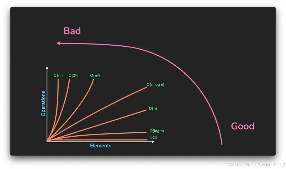
在计算机科学的学习过程中,我们常常接触到算法中的大 O 符号。多数人对其的理解较为简单,即越接近
O
(
1
)
O(1)
O(1),复杂度越低,计算越快,性能越好;而越接近
O
(
n
!
)
O(n!)
O(n!),复杂度越高,计算越慢,性能越差。然而,大 O 的定义及其起源却鲜为人知,接下来我们将深入探讨。
大 O 符号的起源
大 O 符号最早由德国数学家**保罗·巴赫曼(Paul Bachmann)**于 1894 年在其著作《解析数论》中首次提出。巴赫曼引入该符号的目的是为了比较和近似表达函数的增长率。此后,**埃德蒙·兰道(Edmund Landau)**进一步完善并推广了这一概念。兰道将其称为“兰道符号(Landau notation)”,而在计算机科学领域,它作为计算算法复杂度的强大工具被广泛使用。除此之外,大 O 符号还有其他变体,例如表示下界的“大 Ω”符号,以及同时表示上下界的“大 Θ”符号。

(华盛顿大学 CSE 373 讲义)
设有两个函数
f
(
n
)
f(n)
f(n) 和
g
(
n
)
g(n)
g(n),若
f
(
n
)
=
O
(
g
(
n
)
)
f(n) = O(g(n))
f(n)=O(g(n)),则意味着对于足够大的
n
n
n,存在一个正常数
C
C
C,使得:
∣
f
(
n
)
∣
≤
C
⋅
∣
g
(
n
)
∣
|f(n)| \leq C \cdot |g(n)|
∣f(n)∣≤C⋅∣g(n)∣
换言之,
f
(
n
)
f(n)
f(n) 可以用
g
(
n
)
g(n)
g(n) 的常数倍来作为上界(upper bound)。
举例来说:
若 f ( n ) = 3 n 2 + 2 n + 1 f(n) = 3n^2 + 2n + 1 f(n)=3n2+2n+1,则 f ( n ) f(n) f(n) 是 O ( n 2 ) O(n^2) O(n2)。因为在分析时,我们仅考虑最高次项 n 2 n^2 n2,并忽略常数系数。
那么,若
f
(
n
)
=
2
n
+
10
f(n) = 2n + 10
f(n)=2n+10 呢?
或许已经猜到,
f
(
n
)
=
O
(
n
)
f(n) = O(n)
f(n)=O(n)。
总之,大 O 符号主要用于表示函数的渐进增长率(asymptotic growth rate)。若觉得这一概念有些晦涩难懂,简单来说,它描述的是随着输入规模增大,函数复杂度的增长情况。
(img ref:EP132: Big O Notation 101: The Secret to Writing Efficient Algorithms)
Big-O 的概念
通常,我们会用 Big-O 来计算两种复杂度:
时间复杂度(Time Complexity)
时间复杂度表示随着输入规模增大,算法执行所需时间(操作次数)的增长率。
常见的时间复杂度
-
O ( 1 ) O(1) O(1) → 常数时间(Constant Time)
示例:通过索引访问数组元素(如 arr[2]),或在哈希表中查找键值(无冲突的情况下)。
解释:与输入规模 n n n 无关,操作一步完成。 -
O ( log n ) O(\log n) O(logn) → 对数时间(Logarithmic Time)
示例:二分查找、平衡二叉搜索树(BST)中查找节点。
解释:每次操作将输入规模减半(例如不断分割数据进行查找)。 -
O ( n ) O(n) O(n) → 线性时间(Linear Time)
示例:遍历数组的所有元素,链表中查找特定值。
解释:操作时间随输入规模 n n n 线性增长。 -
O ( n log n ) O(n \log n) O(nlogn) → 线性对数时间(Linearithmic Time)
示例:归并排序(Merge Sort)、快速排序(Quick Sort)、堆排序(Heap Sort)。
解释:采用分治策略(Divide and Conquer),将 n n n 个元素反复分成两半( log n \log n logn),然后合并( n n n)。 -
O ( n 2 ) O(n^2) O(n2) → 平方时间(Quadratic Time)
示例:嵌套循环检查数组的所有组合(如冒泡排序、选择排序),图中所有节点对的最短路径计算(Floyd-Warshall 算法)。
解释:输入规模增大时,操作时间呈平方级爆炸式增长。 -
O ( 2 n ) O(2^n) O(2n) → 指数时间(Exponential Time)
示例:斐波那契数列的朴素递归实现(重复计算多),生成所有子集(Subset)。
解释:即使输入规模较小,操作时间也呈指数级增长,不实用。
空间复杂度(Space Complexity)
- 空间复杂度表示随着输入规模增大,算法使用的内存增长情况。
常见的空间复杂度
-
O ( 1 ) O(1) O(1) → 常数空间(Constant Space)
示例:单个变量使用(如循环中的索引 i),与输入规模无关的固定大小变量(如 int a = 10)。
解释:与输入规模 n n n 无关,使用固定内存。 -
O ( log n ) O(\log n) O(logn) → 对数空间(Logarithmic Space)
示例:平衡二叉搜索树(BST)的递归遍历(递归调用栈深度),快速排序的平均空间复杂度(分治时栈深度)。
解释:递归或分治算法中,栈 / 内存使用量与输入规模的对数成正比。 -
O ( n ) O(n) O(n) → 线性空间(Linear Space)
示例:存储输入数组的副本(如 newArr = arr.slice()),图的邻接表表示(与节点数成正比的内存)。
解释:内存使用量随输入规模 n n n 线性增长。 -
O ( n 2 ) O(n^2) O(n2) → 平方空间(Quadratic Space)
示例:图的邻接矩阵表示( n × n n \times n n×n 矩阵),动态规划(DP)的二维表(如最长公共子序列)。
解释:内存使用量随输入规模的平方增长,处理大规模数据时效率低下。 -
O ( 2 n ) O(2^n) O(2n) → 指数空间(Exponential Space)
示例:存储所有子集(Subset),递归斐波那契的最差空间复杂度(重复调用栈)。
解释:即使输入规模较小,内存使用量也呈指数级增长。
两者均采用大 O 符号表示,并假设最坏情况(Worst Case)来分类性能。区别在于:时间复杂度关注速度,而空间复杂度关注内存使用。
权衡(Trade-off)
- 快速算法可能消耗更多内存(如动态规划),
- 或者节省内存但增加时间消耗(如递归与迭代对比)。
例如,使用更多内存来降低时间复杂度的一个例子是哈希表。
时间复杂度表 (Time Complexity Table)
| 排序算法 | 最佳情况 (Best) | 平均情况 (Average) | 最差情况 (Worst) |
|---|---|---|---|
| 插入排序 (Insertion Sort) | O ( n ) O(n) O(n) | O ( n 2 ) O(n^2) O(n2) | O ( n 2 ) O(n^2) O(n2) |
| 选择排序 (Selection Sort) | O ( n 2 ) O(n^2) O(n2) | O ( n 2 ) O(n^2) O(n2) | O ( n 2 ) O(n^2) O(n2) |
| 冒泡排序 (Bubble Sort) | O ( n ) O(n) O(n) | O ( n 2 ) O(n^2) O(n2) | O ( n 2 ) O(n^2) O(n2) |
| 归并排序 (Merge Sort) | O ( n log n ) O(n \log n) O(nlogn) | O ( n log n ) O(n \log n) O(nlogn) | O ( n log n ) O(n \log n) O(nlogn) |
| 快速排序 (Quick Sort) | O ( n log n ) O(n \log n) O(nlogn) | O ( n log n ) O(n \log n) O(nlogn) | O ( n 2 ) O(n^2) O(n2) |
| 堆排序 (Heap Sort) | O ( n log n ) O(n \log n) O(nlogn) | O ( n log n ) O(n \log n) O(nlogn) | O ( n log n ) O(n \log n) O(nlogn) |
| 希尔排序 (Shell Sort) | O ( n log n ) O(n \log n) O(nlogn) | O ( n 1.3 ) O(n^{1.3}) O(n1.3) | O ( n 2 ) O(n^2) O(n2) |
| 计数排序 (Counting Sort) | O ( n + k ) O(n + k) O(n+k) | O ( n + k ) O(n + k) O(n+k) | O ( n + k ) O(n + k) O(n+k) |
| 基数排序 (Radix Sort) | O ( n k ) O(nk) O(nk) | O ( n k ) O(nk) O(nk) | O ( n k ) O(nk) O(nk) |
| 桶排序 (Bucket Sort) | O ( n + k ) O(n + k) O(n+k) | O ( n + k ) O(n + k) O(n+k) | O ( n 2 ) O(n^2) O(n2) |
1. 插入排序 (Insertion Sort)
最佳情况 (Best):
O
(
n
)
O(n)
O(n)
当数据已经排序时,每个元素只需比较而无需移动位置。例如:
1
,
2
,
3
,
4
1, 2, 3, 4
1,2,3,4 只需比较,无需插入。
平均情况 (Average):
O
(
n
2
)
O(n^2)
O(n2)
当数据随机分布时,每个元素平均需要移动一半的位置。
最坏情况 (Worst):
O
(
n
2
)
O(n^2)
O(n2)
当数据完全逆序时,每个元素需要与所有前面的元素进行比较和移动。例如:
4
,
3
,
2
,
1
4, 3, 2, 1
4,3,2,1 中,每个元素最多需要
n
n
n 次比较和移动。
2. 选择排序 (Selection Sort)
最佳、平均、最坏情况: 均为
O
(
n
2
)
O(n^2)
O(n2)
原因:无论输入数据的状态如何,每一步都需要在剩余数组中找到最小值(或最大值),因此比较次数始终固定。即使在最佳情况下,交换次数减少,但比较次数不变。
3. 冒泡排序 (Bubble Sort)
最佳情况 (Best):
O
(
n
)
O(n)
O(n)
当数据已经排序时,一次扫描后如果没有发生交换即可提前结束。例如:
1
,
2
,
3
,
4
1, 2, 3, 4
1,2,3,4 不会发生交换,因此只需一次完整扫描后结束。
平均情况 (Average):
O
(
n
2
)
O(n^2)
O(n2)
在随机数据中,每个元素平均需要移动到一半的位置。
最坏情况 (Worst):
O
(
n
2
)
O(n^2)
O(n2)
当数据完全逆序时,每个元素最多需要
n
n
n 次比较和交换。例如:
4
,
3
,
2
,
1
4, 3, 2, 1
4,3,2,1 中,每个元素需要逐个移动。
4. 归并排序 (Merge Sort)
最佳、平均、最坏情况: 均为
O
(
n
log
n
)
O(n \log n)
O(nlogn)
原因:归并排序通过分治法(Divide and Conquer)将数据分为两部分,并在合并过程中始终保持相同的工作量。无论输入数据的状态如何,分治和合并过程都以相同的方式进行。
5. 快速排序 (Quick Sort)
最佳情况 (Best):
O
(
n
log
n
)
O(n \log n)
O(nlogn)
当每次选择的基准值(Pivot)都能将数据均匀划分时,达到平衡划分。例如:
4
,
1
,
3
,
2
,
6
,
5
4, 1, 3, 2, 6, 5
4,1,3,2,6,5 中,基准值为中间值时。
平均情况 (Average):
O
(
n
log
n
)
O(n \log n)
O(nlogn)
大多数情况下,基准值能选择在较为平衡的位置,从而保持
O
(
n
log
n
)
O(n \log n)
O(nlogn) 的性能。
最坏情况 (Worst):
O
(
n
2
)
O(n^2)
O(n2)
当基准值总是选择为最小值或最大值时,导致不平衡划分。例如:
1
,
2
,
3
,
4
,
5
1, 2, 3, 4, 5
1,2,3,4,5 已经排序的数据中,若选择第一个元素为基准值,则每次只划分一侧。
6. 堆排序 (Heap Sort)
最佳、平均、最坏情况: 均为
O
(
n
log
n
)
O(n \log n)
O(nlogn)
原因:堆排序利用堆数据结构提取数据时,始终保持相同的工作量。无论输入数据的状态如何,堆的构建和提取过程都以相同方式进行。
7. 希尔排序 (Shell Sort)
最佳情况 (Best):
O
(
n
log
n
)
O(n \log n)
O(nlogn)
当间隔(Gap)设置合理且数据接近排序状态时效率较高。
平均情况 (Average):
O
(
n
1.3
)
O(n^{1.3})
O(n1.3)
一般情况下,随着间隔逐渐减小,数据逐步排序。
最坏情况 (Worst):
O
(
n
2
)
O(n^2)
O(n2)
当间隔设置不合理或数据完全逆序时效率较低。
8. 计数排序 (Counting Sort)
最佳、平均、最坏情况: 均为
O
(
n
+
k
)
O(n + k)
O(n+k)
原因:当数据范围(
k
k
k)较小时,直接通过计算对数据进行排序,因此无论输入数据状态如何,性能相同。但当
k
k
k 较大时,内存使用量会增加。
9. 基数排序 (Radix Sort)
最佳、平均、最坏情况: 均为
O
(
n
k
)
O(nk)
O(nk)
原因:按位排序时,工作量与数据大小(
n
n
n)和位数(
k
k
k)成正比。无论输入数据状态如何,性能相同。
10. 桶排序 (Bucket Sort)
最佳情况 (Best):
O
(
n
)
O(n)
O(n)
当数据均匀分布且桶内无需排序时。
平均情况 (Average):
O
(
n
+
k
)
O(n + k)
O(n+k)
当数据大致均匀分布,但桶内需要少量排序时。
最坏情况 (Worst):
O
(
n
2
)
O(n^2)
O(n2)
当数据集中在一个桶中时,该桶内的排序成本显著增加。
空间复杂度表 (Space Complexity Table)
| 排序算法 | 最佳情况 (Best) | 平均情况 (Average) | 最差情况 (Worst) |
|---|---|---|---|
| 插入排序 (Insertion Sort) | O ( 1 ) O(1) O(1) | O ( 1 ) O(1) O(1) | O ( 1 ) O(1) O(1) |
| 选择排序 (Selection Sort) | O ( 1 ) O(1) O(1) | O ( 1 ) O(1) O(1) | O ( 1 ) O(1) O(1) |
| 冒泡排序 (Bubble Sort) | O ( 1 ) O(1) O(1) | O ( 1 ) O(1) O(1) | O ( 1 ) O(1) O(1) |
| 归并排序 (Merge Sort) | O ( n ) O(n) O(n) | O ( n ) O(n) O(n) | O ( n ) O(n) O(n) |
| 快速排序 (Quick Sort) | O ( log n ) O(\log n) O(logn) | O ( log n ) O(\log n) O(logn) | O ( n ) O(n) O(n) |
| 堆排序 (Heap Sort) | O ( 1 ) O(1) O(1) | O ( 1 ) O(1) O(1) | O ( 1 ) O(1) O(1) |
| 希尔排序 (Shell Sort) | O ( 1 ) O(1) O(1) | O ( 1 ) O(1) O(1) | O ( 1 ) O(1) O(1) |
| 计数排序 (Counting Sort) | O ( k ) O(k) O(k) | O ( k ) O(k) O(k) | O ( k ) O(k) O(k) |
| 基数排序 (Radix Sort) | O ( n + k ) O(n + k) O(n+k) | O ( n + k ) O(n + k) O(n+k) | O ( n + k ) O(n + k) O(n+k) |
| 桶排序 (Bucket Sort) | O ( n + k ) O(n + k) O(n+k) | O ( n + k ) O(n + k) O(n+k) | O ( n 2 ) O(n^2) O(n2) |
1. 插入排序、选择排序、冒泡排序、堆排序、希尔排序
这些均为原地(In-place)排序算法,几乎不需要额外的内存。空间复杂度始终为 O ( 1 ) O(1) O(1)。
2. 归并排序
需要额外的数组来存储分治后的子数组。空间复杂度始终为 O ( n ) O(n) O(n),这是归并排序的主要缺点之一。
3. 快速排序
由于递归调用栈的存在,需要额外的内存。平均情况下需要 O ( log n ) O(\log n) O(logn) 的空间,而在最坏情况下可能增加到 O ( n ) O(n) O(n)。
4. 计数排序
根据数据范围( k k k)需要额外的内存。空间复杂度为 O ( k ) O(k) O(k)。
5. 基数排序
按照每个位数进行排序,因此需要与数据大小( n n n)和范围( k k k)成比例的额外内存。空间复杂度为 O ( n + k ) O(n + k) O(n+k)。
6. 桶排序
将数据分配到桶中存储,因此需要与数据大小和桶的数量成比例的额外内存。空间复杂度为
O
(
n
+
k
)
O(n + k)
O(n+k)。
But, this article is not intended to sort the Big-O of sorting algorithms from a mathematical perspective, but to illustrate the limitations of Big-O.
但是,本文并不打算从数学角度对排序算法中的 Big-O 进行排序,而是要说明 Big-O 的局限性。

All models are wrong, but some are useful.
——George Edward Pelham Box, mathematician
Big-O is a simplified complexity model that cannot encompass all variables in reality. It is merely a way to quickly compare algorithm efficiency.
大 O 是一个简化的复杂性模型,在现实中不能包含所有变量。它只是一种快速比较算法效率的方法。
Let us consider an example.
Big-O 的局限性
1. Big-O 基于最坏情况(Worst Case)
using System;
using System.Diagnostics;

class QuickSortExample
{
    // 最坏情况(已排序数组)
    static int[] QuickSortWorst(int[] arr)
    {
        if (arr.Length <= 1)
            return arr;

        int pivot = arr[0];  // 选择第一个元素作为基准点(引发最坏情况)
        var left = Array.FindAll(arr, x => x <= pivot);
        var right = Array.FindAll(arr, x => x > pivot);
        return Concatenate(QuickSortWorst(left), pivot, QuickSortWorst(right));
    }

    // 平均情况(随机基准点)
    static int[] QuickSortAvg(int[] arr)
    {
        if (arr.Length <= 1)
            return arr;

        int pivot = arr[arr.Length / 2];  // 选择中间元素作为基准点
        var left = Array.FindAll(arr, x => x < pivot);
        var middle = Array.FindAll(arr, x => x == pivot);
        var right = Array.FindAll(arr, x => x > pivot);
        return Concatenate(QuickSortAvg(left), middle, QuickSortAvg(right));
    }

    // 数组连接辅助函数
    static int[] Concatenate(int[] left, int pivot, int[] right)
    {
        var result = new int[left.Length + 1 + right.Length];
        Array.Copy(left, result, left.Length);
        result[left.Length] = pivot;
        Array.Copy(right, 0, result, left.Length + 1, right.Length);
        return result;
    }

    static void Main()
    {
        int[] arrSorted = new int[1000];  // 已排序数组(最坏情况)
        for (int i = 0; i < arrSorted.Length; i++)
            arrSorted[i] = i;

        int[] arrRandom = new int[1000];  // 随机数组
        Random rand = new Random();
        for (int i = 0; i < arrRandom.Length; i++)
            arrRandom[i] = rand.Next(1000);

        // 测量最坏情况的时间
        var stopwatch = Stopwatch.StartNew();
        QuickSortWorst(arrSorted);
        Console.WriteLine($"最坏情况: {stopwatch.Elapsed.TotalMilliseconds}ms");

        // 测量平均情况的时间
        stopwatch.Restart();
        QuickSortAvg(arrRandom);
        Console.WriteLine($"平均情况: {stopwatch.Elapsed.TotalMilliseconds}ms");
    }
}
例如,快速排序在平均情况下是 O ( n log n ) O(n \log n) O(nlogn),但在最坏情况下是 O ( n 2 ) O(n^2) O(n2)。根据 Big-O 的定义,它会被标记为 O ( n 2 ) O(n^2) O(n2)。然而,在实际编程中,快速排序的表现往往优于理论上的最坏情况。此外, O ( n 2 ) O(n^2) O(n2) 的算法在某些情况下可能比 O ( n log n ) O(n \log n) O(nlogn) 更快,尤其是在小规模数据中,由于缓存局部性(cache locality)的原因。
2. 忽略常数因子(Constant Factor)
using System;
using System.Diagnostics;

class ConstantCoefficientExample
{
    static int F(int n)
    {
        return 100 * n + 1000;  // $O(n)$
    }

    static int G(int n)
    {
        return (int)(0.1 * n * n);  // $O(n^2)$
    }

    static void Main()
    {
        int n = 10;  // 小输入规模
        var stopwatch = Stopwatch.StartNew();
        F(n);
        Console.WriteLine($"$O(n)$ 函数执行时间: {stopwatch.Elapsed.TotalMilliseconds}ms");
        stopwatch.Restart();
        G(n);
        Console.WriteLine($"$O(n^2)$ 函数执行时间: {stopwatch.Elapsed.TotalMilliseconds}ms");
    }
}
例如,如果有两个函数 f ( n ) = 100 n + 1000 f(n) = 100n + 1000 f(n)=100n+1000 和 g ( n ) = 0.1 n 2 g(n) = 0.1n^2 g(n)=0.1n2,Big-O 会将它们分别归类为 O ( n ) O(n) O(n) 和 O ( n 2 ) O(n^2) O(n2)。但在小规模 n n n 的情况下, g ( n ) g(n) g(n) 可能会更快。
3. 相同复杂度也可能有性能差异
快速排序示例代码 (QuickSort Example)
using System;
using System.Diagnostics;

class QuickSortExample
{
    static void QuickSort(int[] arr, int left, int right)
    {
        if (left < right)
        {
            int pivotIndex = Partition(arr, left, right);
            QuickSort(arr, left, pivotIndex - 1);  // 对左子数组进行排序
            QuickSort(arr, pivotIndex + 1, right); // 对右子数组进行排序
        }
    }

    static int Partition(int[] arr, int left, int right)
    {
        int pivot = arr[right];  // 选择基准点(这里选择最后一个元素)
        int i = left - 1;
        for (int j = left; j < right; j++)
        {
            if (arr[j] < pivot)
            {
                i++;
                Swap(arr, i, j);
            }
        }
        Swap(arr, i + 1, right);  // 将基准点移动到正确位置
        return i + 1;
    }

    static void Swap(int[] arr, int i, int j)
    {
        int temp = arr[i];
        arr[i] = arr[j];
        arr[j] = temp;
    }

    static void Main()
    {
        int[] arr = { 3, 6, 8, 10, 1, 2, 1 };
        Console.WriteLine("排序前: " + string.Join(", ", arr));
        var stopwatch = Stopwatch.StartNew();
        QuickSort(arr, 0, arr.Length - 1);
        Console.WriteLine($"快速排序时间: {stopwatch.Elapsed.TotalMilliseconds}ms");
        Console.WriteLine("排序后: " + string.Join(", ", arr));
    }
}
堆排序示例代码 (HeapSort Example)
using System;
using System.Diagnostics;

class HeapSortExample
{
    static void HeapSort(int[] arr)
    {
        int n = arr.Length;
        // 构建最大堆
        for (int i = n / 2 - 1; i >= 0; i--)
            Heapify(arr, n, i);
        // 从堆中逐个提取元素
        for (int i = n - 1; i > 0; i--)
        {
            Swap(arr, 0, i);  // 将根节点(最大值)与最后一个元素交换
            Heapify(arr, i, 0);  // 缩小堆大小并重新构建堆
        }
    }

    static void Heapify(int[] arr, int n, int i)
    {
        int largest = i;  // 父节点
        int left = 2 * i + 1;  // 左子节点
        int right = 2 * i + 2; // 右子节点
        // 如果左子节点更大
        if (left < n && arr[left] > arr[largest])
            largest = left;
        // 如果右子节点更大
        if (right < n && arr[right] > arr[largest])
            largest = right;
        // 如果最大值不是父节点
        if (largest != i)
        {
            Swap(arr, i, largest);
            Heapify(arr, n, largest);  // 递归地调整子树
        }
    }

    static void Swap(int[] arr, int i, int j)
    {
        int temp = arr[i];
        arr[i] = arr[j];
        arr[j] = temp;
    }

    static void Main()
    {
        int[] arr = { 3, 6, 8, 10, 1, 2, 1 };
        Console.WriteLine("排序前: " + string.Join(", ", arr));
        var stopwatch = Stopwatch.StartNew();
        HeapSort(arr);
        Console.WriteLine($"堆排序时间: {stopwatch.Elapsed.TotalMilliseconds}ms");
        Console.WriteLine("排序后: " + string.Join(", ", arr));
    }
}
排序比较代码 (SortComparison)
using System;
using System.Diagnostics;

class SortComparison
{
    static void Main()
    {
        int[] arr = new int[100000];
        Random rand = new Random();
        for (int i = 0; i < arr.Length; i++)
            arr[i] = rand.Next(100000);
        // 测量快速排序的时间
        var stopwatch = Stopwatch.StartNew();
        QuickSort((int[])arr.Clone(), 0, arr.Length - 1);
        Console.WriteLine($"快速排序时间: {stopwatch.Elapsed.TotalMilliseconds}ms");
        // 测量堆排序的时间
        stopwatch.Restart();
        HeapSort((int[])arr.Clone());
        Console.WriteLine($"堆排序时间: {stopwatch.Elapsed.TotalMilliseconds}ms");
    }

    static void QuickSort(int[] arr, int left, int right)
    {
        if (left < right)
        {
            int pivotIndex = Partition(arr, left, right);
            QuickSort(arr, left, pivotIndex - 1);
            QuickSort(arr, pivotIndex + 1, right);
        }
    }

    static int Partition(int[] arr, int left, int right)
    {
        int pivot = arr[right];
        int i = left - 1;
        for (int j = left; j < right; j++)
        {
            if (arr[j] < pivot)
            {
                i++;
                Swap(arr, i, j);
            }
        }
        Swap(arr, i + 1, right);
        return i + 1;
    }

    static void HeapSort(int[] arr)
    {
        int n = arr.Length;
        for (int i = n / 2 - 1; i >= 0; i--)
            Heapify(arr, n, i);
        for (int i = n - 1; i > 0; i--)
        {
            Swap(arr, 0, i);
            Heapify(arr, i, 0);
        }
    }

    static void Heapify(int[] arr, int n, int i)
    {
        int largest = i;
        int left = 2 * i + 1;
        int right = 2 * i + 2;
        if (left < n && arr[left] > arr[largest])
            largest = left;
        if (right < n && arr[right] > arr[largest])
            largest = right;
        if (largest != i)
        {
            Swap(arr, i, largest);
            Heapify(arr, n, largest);
        }
    }

    static void Swap(int[] arr, int i, int j)
    {
        int temp = arr[i];
        arr[i] = arr[j];
        arr[j] = temp;
    }
}
例如,快速排序和堆排序的理论复杂度相同,但由于堆排序的常数因子较大且缓存效率较低,因此在实际应用中通常比快速排序慢。此外,输入数据的特性、错误数据、输入规模等因素都会导致实际表现与 Big-O 不符。硬件环境和缓存局部性等问题也会导致性能差异。正如我之前的文章提到的,即使是相同的复杂度,仅仅是因为双重循环是以行优先还是列优先的方式进行,缓存未命中率的不同也会导致速度差异。
结论
Big-O 是一个非常强大的工具,但它并不是万能的。我们不能盲目崇拜理论,认为它可以解决一切问题。现实世界的问题总是复杂多样的,理论只是现实的一部分抽象。因此,我们应该将理论作为解决问题的指南针,但也要注意观察周围的“风景”,确保我们走在正确的道路上。
via:
-
Big O notation.doc - big_o.pdf
https://web.mit.edu/course/16/16.070/www/lecture/big_o.pdf -
A beginner’s guide to Big O Notation - Rob Bell
https://robbell.io/2009/06/a-beginners-guide-to-big-o-notation -
大 O 符号 - 维基百科,自由的百科全书
https://zh.wikipedia.org/wiki/大O符号 -
Big-O 表示法简介(基础入门)-优快云博客
https://blog.youkuaiyun.com/2404_84768005/article/details/145666513 -
big O notation - 大 O 表示法-优快云博客
https://blog.youkuaiyun.com/chengyq116/article/details/113746736 -
大O表示法入门-优快云博客
https://blog.youkuaiyun.com/yuhk231/article/details/60099774


 653
653

 被折叠的 条评论
为什么被折叠?
被折叠的 条评论
为什么被折叠?
 到【灌水乐园】发言


