


注:本文为 “混沌理论” 相关合辑。
英文引文,机翻未校。
中文引文,略作重排。
如有内容异常,请看原文。
A brief history of chaos
混沌简史
Laws of attribution
归属法则
-
Arnol’d’s Law: everything that is discovered is named after someone else (including Arnol’d’s law)
阿诺尔德法则:所有发现都以他人之名命名(包括阿诺尔德法则本身)。
-
Berry’s Law: sometimes, the sequence of antecedents seems endless. So, nothing is discovered for the first time.
贝里法则:有时,先驱者的序列似乎无穷无尽。因此,没有任何事物是首次被发现的。
-
Whiteheads’s Law: Everything of importance has been said before by someone who did not discover it. -Sir Michael V. Berry
怀特海法则:所有重要的事物都曾被未曾发现它的人说过。 —— 迈克尔・V・贝里爵士
Writing a history of anything is a reckless undertaking, especially a history of something that has preoccupied at one time or other any serious thinker from ancient Sumer to today’s Hong Kong. A mathematician, to take an example, might see it this way: “History of dynamical systems.” Nevertheless, here comes yet another very imperfect attempt.
撰写任何事物的历史都是一项鲁莽的尝试,尤其是撰写一个从古代苏美尔到今日香港的所有严肃思想家都曾关注过的主题的历史。举例来说,数学家可能会称之为 “动力系统史”。尽管如此,这里仍将呈现另一次极不完美的尝试。
A1.1 Chaos is born
A1.1 混沌的诞生
I’ll maybe discuss more about its history when I learn more about it. -Maciej Zworski
“或许当我对其有更多了解后,会再深入探讨它的历史。”—— 马切伊・兹沃尔斯基
(R. Mainieri and P. Cvitanovi´c) Trying to predict the motion of the Moon has preoccupied astronomers since antiquity. Accurate understanding of its motion was important for determining the longitude of ships while traversing open seas.
(R. 迈尼耶里与 P. 茨维坦诺维奇)自古以来,预测月球运动一直是天文学家关注的焦点。准确理解月球运动对于船舶在公海上确定经度至关重要。
Kepler’s Rudolphine tables had been a great improvement over previous tables, and Kepler was justly proud of his achievements. He wrote in the introduction to the announcement of Kepler’s third law, Harmonice Mundi (Linz, 1619) in a style that would not fly with the contemporary Physical Review Letters editors:
开普勒的《鲁道夫星表》较之前的星表有了重大改进,他也理应为自己的成就感到自豪。在其宣布开普勒第三定律的著作《世界和谐》(林茨,1619 年)的引言中,他以一种不符合当代《物理评论快报》编辑风格的笔触写道:
What I prophesied two-and-twenty years ago, as soon as I discovered the five solids among the heavenly orbits–what I firmly believed long before I had seen Ptolemy’s Harmonics–what I had promised my friends in the title of this book, which I named before I was sure of my discovery–what sixteen years ago, I urged as the thing to be sought–that for which I joined Tycho Brahe, for which I settled in Prague, for which I have devoted the best part of my life to astronomical contemplations, at length I have brought to light, and recognized its truth beyond my most sanguine expectations. It is not eighteen months since I got the first glimpse of light, three months since the dawn, very few days since the unveiled sun, most admirable to gaze upon, burst upon me. Nothing holds me; I will indulge my sacred fury; I will triumph over mankind by the honest confession that I have stolen the golden vases of the Egyptians to build up a tabernacle for my God far away from the confines of Egypt. If you forgive me, I rejoice; if you are angry, I can bear it; the die is cast, the book is written, to be read either now or in posterity, I care not which; it may well wait a century for a reader, as God has waited six thousand years for an observer.
“22 年前,当我在天体轨道中发现那五个正多面体时,我就预言过 —— 在看到托勒密的《和谐论》之前很久我就坚信不疑 —— 我在这本书的标题中向朋友们承诺过(我在确定发现之前就已命名)——16 年前我就极力主张去探寻的东西 —— 为此我加入第谷・布拉赫的团队,为此我定居布拉格,为此我将毕生最美好的时光投入天文观测 —— 最终,我将其公之于世,并认识到其真实性远超我最乐观的预期。距我初窥曙光不过 18 个月,距黎明不过 3 个月,而那令人惊叹的、揭开面纱的太阳照耀我的日子更是屈指可数。没有什么能束缚我;我将放纵我神圣的狂热;我要坦然承认,我偷了埃及人的金罐,为我的上帝在远离埃及边界之处建造会幕,以此战胜世人。若你宽恕我,我欣喜;若你愤怒,我承受;木已成舟,书已写成,无论现在还是后世有人阅读,我都不在意;它大可以等待一个世纪才遇到读者,就像上帝等待了六千年才遇到一个观测者。”
Then came Newton. Classical mechanics has not stood still since Newton. The formalism that we use today was developed by Euler and Lagrange. By the end of the 1800’s the three problems that would lead to the notion of chaotic dynamics were already known: the three-body problem, the ergodic hypothesis, and nonlinear oscillators.
随后牛顿登场。自牛顿以来,经典力学从未停滞不前。我们如今使用的形式体系由欧拉和拉格朗日发展而来。到 19 世纪末,引发混沌动力学概念的三个问题已为人所知:三体问题、遍历假说和非线性振荡器。
A1.1.1 Three-body problem
A1.1.1 三体问题
Bernoulli used Newton’s work on mechanics to derive the elliptic orbits of Kepler and set an example of how equations of motion could be solved by integrating. But the motion of the Moon is not well approximated by an ellipse with the Earth at a focus; at least the effects of the Sun have to be taken into account if one wants to reproduce the data the classical Greeks already possessed. To do that one has to consider the motion of three bodies: the Moon, the Earth, and the Sun. When the planets are replaced by point particles of arbitrary masses, the problem to be solved is known as the three-body problem. The three-body problem was also a model to another concern in astronomy. In the Newtonian model of the solar system it is possible for one of the planets to go from an elliptic orbit around the Sun to an orbit that escaped its dominion or that plunged right into it. Knowing if any of the planets would do so became the problem of the stability of the solar system. A planet would not meet this terrible end if solar system consisted of two celestial bodies, but whether such fate could befall in the three-body case remained unclear.
伯努利利用牛顿的力学成果推导出开普勒椭圆轨道,并展示了如何通过积分求解运动方程。但月球的运动并不能用以地球为焦点的椭圆来很好地近似;若要重现古希腊人已掌握的数据,至少必须考虑太阳的影响。为此,需研究三个天体的运动:月球、地球和太阳。当行星被替换为任意质量的质点时,所要解决的问题即三体问题。三体问题也是天文学中另一个关注点的模型:在太阳系的牛顿模型中,某颗行星可能从绕太阳的椭圆轨道变为逃逸轨道或坠入太阳的轨道。判断是否有行星会如此运动,即太阳系稳定性问题。若太阳系仅含两个天体,行星不会遭遇此厄运,但三体情形下是否会有此命运仍不明确。
After many failed attempts to solve the three-body problem, natural philosophers started to suspect that it was impossible to integrate. The usual technique for integrating problems was to find the conserved quantities, quantities that do not change with time and allow one to relate the momenta and positions at different times. The first sign on the impossibility of integrating the three-body problem came from a result of Bruns that showed that there were no conserved quantities that were polynomial in the momenta and positions. Bruns’ result did not preclude the possibility of more complicated conserved quantities. This problem was settled by Poincar´e and Sundman in two very different ways [A1.1, A1.2].
在多次尝试求解三体问题失败后,自然哲学家开始怀疑其不可积。积分问题的常用方法是寻找守恒量 —— 不随时间变化且能关联不同时刻动量与位置的量。布伦斯的研究首次表明三体问题不可积:不存在关于动量和位置的多项式守恒量。但布伦斯的结果并未排除更复杂守恒量的存在性。这一问题由庞加莱和桑德曼以两种截然不同的方式解决 [A1.1, A1.2]。
In an attempt to promote the journal Acta Mathematica, Mittag-Leffler got the permission of the King Oscar II of Sweden and Norway to establish a mathematical competition. Several questions were posed (although the king would have preferred only one), and the prize of 2500 kroner would go to the best submission. One of the questions was formulated by Weierstrass:
为推广《数学学报》,米塔格 - 列夫勒获得瑞典 - 挪威国王奥斯卡二世的许可,设立了一项数学竞赛。竞赛提出了若干问题(尽管国王更希望只有一个),最佳答案将获得 2500 克朗奖金。其中一个问题由魏尔斯特拉斯提出:
Given a system of arbitrary mass points that attract each other according to Newton’s laws, under the assumption that no two points ever collide, try to find a representation of the coordinates of each point as a series in a variable that is some known function of time and for all of whose values the series converges uniformly. This problem, whose solution would considerably extend our understanding of the solar system, …
“给定一组任意质点,它们根据牛顿定律相互吸引,假设任意两点永不碰撞,试将每个质点的坐标表示为某个变量的级数,该变量是时间的已知函数,且级数对所有变量值均一致收敛。解决此问题将极大地拓展我们对太阳系的理解……”
Poincar´e’s submission won the prize. He showed that conserved quantities that were analytic in the momenta and positions could not exist. To show that he introduced methods that were very geometrical in spirit: the importance of state space flow, the role of periodic orbits and their cross sections, the homoclinic points.
庞加莱的投稿获奖。他证明了不存在关于动量和位置的解析守恒量。为此,他引入了极具几何思想的方法:状态空间流的重要性、周期轨道及其截面的作用、同宿点等。
The interesting thing about Poincar´e’s work was that it did not solve the problem posed. He did not find a function that would give the coordinates as a function of time for all times. He did not show that it was impossible either, but rather that it could not be done with the Bernoulli technique of finding a conserved quantity and trying to integrate. Integration would seem unlikely from Poincar´e’s prizewinning memoir, but it was accomplished by the Finnish-born Swedish mathematician Sundman. Sundman showed that to integrate the three-body problem one had to confront the two-body collisions. He did that by making them go away through a trick known as regularization of the collision manifold. The trick is not to expand the coordinates as a function of time t t t, but rather as a function of t 3 \sqrt [3]{t} 3t. To solve the problem for all times he used a conformal map into a strip. This allowed Sundman to obtain a series expansion for the coordinates valid for all times, solving the problem that was proposed by Weirstrass in the King Oscar II’s competition.
庞加莱工作的有趣之处在于,他并未解决所提出的问题。他既未找到能给出所有时刻坐标作为时间函数的表达式,也未证明其不可能,而是表明无法用伯努利那种寻找守恒量并积分的方法解决。从庞加莱的获奖论文看,积分似乎无望,但出生于芬兰的瑞典数学家桑德曼却完成了这一工作。桑德曼指出,要积分三体问题必须处理两体碰撞,并通过碰撞流形正则化的技巧消除碰撞:不将坐标展开为时间 t t t 的函数,而是展开为 t 3 \sqrt [3]{t} 3t 的函数。为求解所有时刻的问题,他使用了到带状区域的共形映射。这使桑德曼得到了对所有时间均有效的坐标级数展开,解决了魏尔斯特拉斯在奥斯卡二世竞赛中提出的问题。
The Sundman’s series are not used today to compute the trajectories of any three-body system. That is more simply accomplished by numerical methods or through series that, although divergent, produce better numerical results. The conformal map and the collision regularization mean that the series are effectively in the variable 1 − e − t 3 1 - e^{-\sqrt [3]{t}} 1−e−3t. Quite rapidly this gets exponentially close to one, the radius of convergence of the series. Many terms, more terms than any one has ever wanted to compute, are needed to achieve numerical convergence. Though Sundman’s work deserves better credit than it gets, it did not live up to Weirstrass’s expectations, and the series solution did not “considerably extend our understanding of the solar system.’ The work that followed from Poincar´e did.
如今,桑德曼级数并未用于计算任何三体系统的轨迹。这一任务更简单地通过数值方法或虽发散但数值结果更好的级数完成。共形映射和碰撞正则化意味着级数实际上以变量 1 − e − t 3 1 - e^{-\sqrt [3]{t}} 1−e−3t 展开,该变量会迅速指数级逼近级数的收敛半径 1。要实现数值收敛,需要计算极多项 —— 多到没人愿意尝试。尽管桑德曼的工作值得更多认可,但它并未达到魏尔斯特拉斯的预期,其级数解也未 “极大地拓展我们对太阳系的理解”。而庞加莱后续的工作做到了这一点。
A1.1.2 Ergodic hypothesis
A1.1.2 遍历假说
The second problem that played a key role in development of chaotic dynamics was the ergodic hypothesis of Boltzmann. Maxwell and Boltzmann had combined the mechanics of Newton with notions of probability in order to create statistical mechanics, deriving thermodynamics from the equations of mechanics. To evaluate the heat capacity of even a simple system, Boltzmann had to make a great simplifying assumption of ergodicity: that the dynamical system would visit every part of the phase space allowed by conservation laws equally often. This hypothesis was extended to other averages used in statistical mechanics and was called the ergodic hypothesis. It was reformulated by Poincar´e to say that a trajectory comes as close as desired to any phase space point.
在混沌动力学发展中起关键作用的第二个问题是玻尔兹曼的遍历假说。麦克斯韦和玻尔兹曼将牛顿力学与概率概念结合,创立了统计力学,从力学方程推导出热力学。为计算即使是简单系统的热容,玻尔兹曼不得不做出遍历性这一重大简化假设:动力系统会以相同频率遍历守恒律所允许的相空间的每一部分。这一假设被推广到统计力学中使用的其他平均值,称为遍历假说。庞加莱将其重新表述为:轨迹会无限接近相空间中的任意点。
Proving the ergodic hypothesis turned out to be very difficult. By the end of twentieth century it has only been shown true for a few systems and wrong for quite a few others. Early on, as a mathematical necessity, the proof of the hypothesis was broken down into two parts. First one would show that the mechanical system was ergodic (it would go near any point) and then one would show that it would go near each point equally often and regularly so that the computed averages made mathematical sense. Koopman took the first step in proving the ergodic hypothesis when he realized that it was possible to reformulate it using the recently developed methods of Hilbert spaces [A1.3]. This was an important step that showed that it was possible to take a finite-dimensional nonlinear problem and reformulate it as a infinite-dimensional linear problem. This does not make the problem easier, but it does allow one to use a different set of mathematical tools on the problem. Shortly after Koopman started lecturing on his method, von Neumann proved a version of the ergodic hypothesis, giving it the status of a theorem [A1.4]. He proved that if the mechanical system was ergodic, then chapter 19 the computed averages would make sense. Soon afterwards Birkhoff published a much stronger version of the theorem.
证明遍历假说极具难度。到 20 世纪末,仅证明其对少数系统成立,对更多系统不成立。早期,出于数学必要性,假说的证明被分为两部分:首先证明力学系统是遍历的(会接近任意点),然后证明其以相同频率且规则地接近各点,使计算出的平均值具有数学意义。柯普曼迈出了证明遍历假说的第一步,他意识到可利用新近发展的希尔伯特空间方法重新表述假说 [A1.3]。这一重要步骤表明,有限维非线性问题可重新表述为无穷维线性问题。这并未简化问题,但允许使用另一套数学工具。在柯普曼开始讲授其方法后不久,冯・诺依曼证明了遍历假说的一个版本,使其成为定理 [A1.4]。他证明,若力学系统是遍历的,则第 19 章中计算的平均值是有意义的。不久后,伯克霍夫发表了该定理的一个更强版本。
A1.1.3 Nonlinear oscillators
A1.1.3 非线性振荡器
The third problem that was very influential in the development of the theory of chaotic dynamical systems was the work on the nonlinear oscillators. The problem is to construct mechanical models that would aid our understanding of physical systems. Lord Rayleigh came to the problem through his interest in understanding how musical instruments generate sound. In the first approximation one can construct a model of a musical instrument as a linear oscillator. But real instruments do not produce a simple tone forever as the linear oscillator does, so Lord Rayleigh modified this simple model by adding friction and more realistic models for the spring. By a clever use of negative friction he created two basic models for the musical instruments. These models have more than a pure tone and decay with time when not stroked. In his book The Theory of Sound Lord Rayleigh introduced a series of methods that would prove quite general, such as the notion of a limit cycle, a periodic motion a system goes to regardless of the initial conditions.
对混沌动力系统理论发展影响深远的第三个问题是关于非线性振荡器的研究。其目标是构建有助于理解物理系统的力学模型。瑞利勋爵因对乐器发声原理的兴趣涉足此问题。一级近似下,乐器可建模为线性振荡器,但真实乐器不会像线性振荡器那样永远产生单一音调,因此瑞利勋爵通过添加摩擦和更真实的弹簧模型对其进行修正。他巧妙利用负摩擦,为乐器创建了两个基本模型。这些模型产生的并非纯音,且在不被激发时会随时间衰减。在《声学理论》一书中,瑞利勋爵引入了一系列具有普适性的方法,例如极限环概念 —— 系统无论初始条件如何都会趋向的周期性运动。
A1.2 Chaos grows up
A1.2 混沌的发展
(R. Mainieri)
(R. 迈尼耶里)
The theorems of von Neumann and Birkhoff on the ergodic hypothesis were published in 1912 and 1913. This line of enquiry developed in two directions. One direction took an abstract approach and considered dynamical systems as transformations of measurable spaces into themselves. Could we classify these transformations in a meaningful way? This lead Kolmogorov to the introduction of the concept of entropy for dynamical systems. With entropy as a dynamical invariant it became possible to classify a set of abstract dynamical systems known as the Bernoulli systems. The other line that developed from the ergodic hypothesis was in trying to find mechanical systems that are ergodic. An ergodic system could not have stable orbits, as these would break ergodicity. So in 1898 Hadamard published a paper with a playful title of ‘… billiards …,’ where he showed that the motion of balls on surfaces of constant negative curvature is everywhere unstable. This dynamical system was to prove very useful and it was taken up by Birkhoff. Morse in 1923 showed that it was possible to enumerate the orbits of a ball on a surface of constant negative curvature. He did this by introducing a symbolic code to each orbit and showed that the number of possible codes grew exponentially with the length of the code. With contributions by Artin, Hedlund, and H. Hopf it was eventually proven that the motion of a ball on a surface of constant negative curvature was ergodic. The importance of this result escaped most physicists, one exception being Krylov, who understood that a physical billiard was a dynamical system on a surface of negative curvature, but with the curvature concentrated along the lines of collision. Sinai, who was the first to show that a physical billiard can be ergodic, knew Krylov’s work well.
冯・诺依曼和伯克霍夫关于遍历假说的定理发表于 1912 年和 1913 年。这一研究方向分化为两条支线:一条采用抽象方法,将动力系统视为可测空间到自身的变换,探索这些变换的有意义分类方式。这促使柯尔莫哥洛夫引入动力系统的熵概念,以熵作为动力学不变量,成功对一类称为伯努利系统的抽象动力系统进行分类。另一条支线源于遍历假说,旨在寻找遍历的力学系统。遍历系统不可能有稳定轨道,因为稳定轨道会破坏遍历性。1898 年,阿达马发表了一篇标题诙谐的论文《…… 台球……》,证明常负曲率表面上球的运动处处不稳定。这一动力系统后来被证明非常有用,并被伯克霍夫采纳。1923 年,莫尔斯表明可枚举常负曲率表面上球的轨道:他为每个轨道引入符号编码,并证明可能的编码数量随编码长度呈指数增长。在阿廷、赫德伦德和 H. 霍普夫的贡献下,最终证明常负曲率表面上球的运动是遍历的。大多数物理学家未意识到这一结果的重要性,但克里洛夫除外,他认识到物理台球是负曲率表面上的动力系统,但其曲率集中在碰撞线上。西奈是首个证明物理台球可具有遍历性的人,他深谙克里洛夫的工作。
The work of Lord Rayleigh also received vigorous development. It prompted many experiments and some theoretical development by van der Pol, Duffing, and Hayashi. They found other systems in which the nonlinear oscillator played a role and classified the possible motions of these systems. This concreteness of experiments, and the possibility of analysis was too much of temptation for Mary Lucy Cartwright and J.E. Littlewood [A1.5], who set out to prove that many of the structures conjectured by the experimentalists and theoretical physicists did indeed follow from the equations of motion. Birkhoff had found a ‘remarkable curve’ in a two dimensional map; it appeared to be non-differentiable and it would be nice to see if a smooth flow could generate such a curve. The work of Cartwright and Littlewood lead to the work of Levinson, which in turn provided the basis for the horseshoe construction of S. Smale. chapter 15
瑞利勋爵的工作也得到了蓬勃发展。它促使范德波尔、杜芬和林忠四郎开展了大量实验和理论研究。他们发现了其他非线性振荡器起作用的系统,并对这些系统的可能运动进行了分类。实验的具体性和可分析性吸引了玛丽・露西・卡特赖特和 J.E. 利特尔伍德 [A1.5],他们着手证明实验者和理论物理学家推测的许多结构确实源于运动方程。伯克霍夫在二维映射中发现了一条 “奇异曲线”,它似乎不可微,人们好奇光滑流是否能生成此类曲线。卡特赖特和利特尔伍德的工作启发了莱文森,而莱文森的工作又为 S. 斯梅尔的马蹄构造奠定了基础(第 15 章)。
In Russia, Lyapunov paralleled the methods of Poincar´e and initiated the strong Russian dynamical systems school [A1.6]. Andronov carried on with the study of nonlinear oscillators and in 1937 introduced together with Pontryagin the notion of coarse systems. They were formalizing the understanding garnered from the study of nonlinear oscillators, the understanding that many of the details on how these oscillators work do not affect the overall picture of the state space: there will still be limit cycles if one changes the dissipation or spring force function by a little bit. And changing the system a little bit has the great advantage of eliminating exceptional cases in the mathematical analysis. Coarse systems were the concept that caught Smale’s attention and enticed him to study dynamical systems.
在俄罗斯,李雅普诺夫与庞加莱的方法并行,开创了强大的俄罗斯动力系统学派 [A1.6]。安德罗诺夫继续研究非线性振荡器,并于 1937 年与庞特里亚金共同引入粗系统的概念。他们将对非线性振荡器的理解形式化:振荡器工作方式的许多细节并不影响状态空间的整体图景 —— 即使轻微改变耗散或弹簧力函数,极限环仍然存在。轻微改变系统还有一个巨大优势,即消除数学分析中的例外情况。粗系统这一概念引起了斯梅尔的关注,促使他研究动力系统。
A1.3 Chaos with us
A1.3 混沌的现状
(R. Mainieri)
(R. 迈尼耶里)
In the fall of 1961 Steven Smale was invited to Kiev where he met Arnol’d, Anosov, Sinai, and Novikov. He lectured there, and spent a lot of time with Anosov. He suggested a series of conjectures, most of which Anosov proved within a year. It was Anosov who showed that there are dynamical systems for which all points (as opposed to a non–wandering set) admit the hyperbolic structure, and it was in honor of this result that Smale named these systems Axiom-A. In Kiev Smale found a receptive audience that had been thinking about these problems. Smale’s result catalyzed their thoughts and initiated a chain of developments that persisted into the 1970’s.
1961 年秋,史蒂文・斯梅尔应邀前往基辅,在那里他会见了阿诺尔德、阿诺索夫、西奈和诺维科夫。他在那里授课,并与阿诺索夫长时间交流。他提出了一系列猜想,其中大多数由阿诺索夫在一年内证明。阿诺索夫证明了存在所有点(而非非游荡集)都具有双曲结构的动力系统,斯梅尔为纪念这一成果,将这些系统命名为 A 公理系统。在基辅,斯梅尔遇到了对这些问题早有思考的知音。他的成果激发了他们的思考,引发了持续到 20 世纪 70 年代的一系列发展。
Smale collected his results and their development in the 1967 review article on dynamical systems, entitled “Differentiable dynamical systems” [A1.7]. There are chapter 15 many great ideas in this paper: the global foliation of invariant sets of the map into disjoint stable and unstable parts; the existence of a horseshoe and enumeration and ordering of all its orbits; the use of zeta functions to study dynamical systems. The emphasis of the paper is on the global properties of the dynamical system, on how to understand the topology of the orbits. Smale’s account takes you from a local differential equation (in the form of vector fields) to the global topological description in terms of horseshoes.
斯梅尔在 1967 年的综述文章《可微动力系统》中总结了他的成果及其发展 [A1.7]。该论文包含诸多重要思想(第 15 章):映射不变集的整体叶状结构分解为不相交的稳定部分和不稳定部分;马蹄的存在性及其所有轨道的枚举与排序;zeta 函数在动力系统研究中的应用。论文重点关注动力系统的整体性质,以及如何理解轨道的拓扑结构。斯梅尔的论述将读者从局部微分方程(以向量场形式)引向基于马蹄的整体拓扑描述。
The path traversed from ergodicity to entropy is a little more confusing. The general character of entropy was understood by Weiner, who seemed to have spoken to Shannon. In 1948 Shannon published his results on information theory, where he discusses the entropy of the shift transformation. Kolmogorov went far beyond and suggested a definition of the metric entropy of an area preserving transformation in order to classify Bernoulli shifts. The suggestion was taken by his student Sinai and the results published in 1959. In 1960 Rohlin connected these results to measure-theoretical notions of entropy. The next step was published in 1965 by Adler and Palis, and also Adler, Konheim, McAndrew; these papers showed that one could define the notion of topological entropy and use it as an invariant to classify continuous maps. In 1967 Anosov and Sinai applied the notion of entropy to the study of dynamical systems. It was in the context of studying the entropy associated to a dynamical system that Sinai introduced Markov partitions in 1968.
从遍历性到熵的发展路径略显曲折。维纳理解了熵的一般特性,他似乎与香农交流过。1948 年,香农发表了信息论成果,其中讨论了移位变换的熵。柯尔莫哥洛夫更进一步,提出了保面积变换的度量熵定义,以分类伯努利移位。他的学生西奈采纳了这一想法,并于 1959 年发表了相关成果。1960 年,罗林将这些成果与熵的测度论概念联系起来。1965 年,阿德勒与帕利斯,以及阿德勒、孔海姆、麦克安德鲁发表的论文迈出了下一步:他们表明可定义拓扑熵概念,并将其作为不变量对连续映射进行分类。1967 年,阿诺索夫和西奈将熵概念应用于动力系统研究。1968 年,西奈在研究动力系统相关熵的背景下引入了马尔可夫分割。
Markov partitions allow one to relate dynamical systems and statistical mechanics; this has been a very fruitful relationship. It adds measure notions to the topological framework laid down in Smale’s paper. Markov partitions divide the state space of the dynamical system into nice little boxes that map into each other. Each box is labeled by a code and the dynamics on the state space maps the codes around, inducing a symbolic dynamics. From the number of boxes needed to cover all the space, Sinai was able to define the notion of entropy of a dynamical system. In 1970 Bowen came up independently with the same ideas, although there was presumably some flow of information back and forth before these papers got published. Bowen also introduced the important concept of shadowing of chaotic orbits. We do not know whether at this point the relations with statistical mechanics were clear to everyone. They became explicit in the work of Ruelle. Ruelle understood that the topology of the orbits could be specified by a symbolic code, and that one could associate an ‘energy’ to each orbit. The energies could be formally combined in a ‘partition function’ to generate the invariant measure of the system.
马尔可夫分割使动力系统与统计力学建立联系,这种联系成果丰硕。它为斯梅尔论文中建立的拓扑框架增添了测度概念。马尔可夫分割将动力系统的状态空间划分为可相互映射的 “良态” 小盒子,每个盒子用一个代码标记,状态空间上的动力学通过映射这些代码诱导出符号动力学。西奈根据覆盖整个空间所需的盒子数量,定义了动力系统的熵概念。1970 年,鲍文独立提出了相同想法,尽管在论文发表前可能存在一些信息交流。鲍文还引入了混沌轨道的跟踪概念。此时,并非所有人都清楚其与统计力学的联系,而吕埃勒的工作明确了这一点。吕埃勒认识到,轨道的拓扑可通过符号编码确定,且可为每个轨道关联一个 “能量”,这些能量可形式上组合为 “配分函数”,以生成系统的不变测度。
After Smale, Sinai, Bowen, and Ruelle had laid the foundations of the statistical mechanics approach to chaotic systems, research turned to studying particular cases. The simplest case to consider is 1-dimensional maps. The topology of the orbits for parabola-like maps was worked out in 1973 by Metropolis, Stein, and Stein [A1.8]. The more general 1-dimensional case was worked out in 1976 by Milnor and Thurston in a widely circulated preprint, whose extended version eventually got published in 1988 [A1.9].
在斯梅尔、西奈、鲍文和吕埃勒奠定了用统计力学方法研究混沌系统的基础后,研究转向具体案例。最简单的案例是一维映射。1973 年,梅特罗波利斯、斯泰因和斯泰因解决了类抛物线映射的轨道拓扑问题 [A1.8]。1976 年,米尔诺和瑟斯顿在一份广泛流传的预印本中解决了更一般的一维情形,其扩展版本最终于 1988 年发表 [A1.9]。
A lecture of Smale and the results of Metropolis, Stein, and Stein inspired Feigenbaum to study simple maps. This lead him to the discovery of the universality in quadratic maps and the application of ideas from field-theory to dynamical systems. Feigenbaum’s work was the culmination in the study of 1-dimensional systems; a complete analysis of a nontrivial transition to chaos. Feigenbaum introduced many new ideas into the field: the use of the renormalization group which led him to introduce functional equations in the study of dynamical systems, the scaling function which completed the link between dynamical systems and statistical mechanics, and the presentation functions which describe the dynamics of scaling functions.
斯梅尔的一次讲座以及梅特罗波利斯、斯泰因和斯泰因的成果启发了费根鲍姆研究简单映射。这使他发现了二次映射中的普适性,并将场论思想应用于动力系统。费根鲍姆的工作是一维系统研究的顶峰,完成了对非平凡混沌 transition 的分析。他为该领域引入了诸多新思想:重正化群的使用(促使他在动力系统研究中引入泛函方程)、完成动力系统与统计力学联系的标度函数,以及描述标度函数动力学的表示函数。
The work in more than one dimension progressed very slowly and is still far from completed. The first result in trying to understand the topology of the orbits in two dimensions (the equivalent of Metropolis, Stein, and Stein, or Milnor and Thurston’s work) was obtained by Thurston. Around 1975 Thurston was giving lectures “On the geometry and dynamics of diffeomorphisms of surfaces.” Thurston’s techniques exposed in that lecture have not been applied in physics, but much of the classification that Thurston developed can be obtained from the notion of a ‘pruning front’ formulated independently by Cvitanovi´c.
高维研究进展缓慢,至今仍远未完成。瑟斯顿取得了理解二维轨道拓扑的首个成果(相当于梅特罗波利斯 - 斯泰因 - 斯泰因或米尔诺 - 瑟斯顿的工作)。1975 年左右,瑟斯顿讲授了《论曲面微分同胚的几何与动力学》。该讲座中提出的技术尚未应用于物理学,但瑟斯顿提出的大部分分类可通过茨维坦诺维奇独立提出的 “修剪前沿” 概念获得。
Once one develops an understanding of the topology of the orbits of a dynamical system, one needs to be able to compute its properties. Ruelle had already generalized the zeta function introduced by Artin and Mazur [A1.10], so that it could be used to compute the average value of observables. The difficulty with Ruelle’s zeta function is that it does not converge very well. Starting out from Smale’s observation that a chaotic dynamical system is dense with a set of periodic orbits, Cvitanovi´c used these orbits as a skeleton on which to evaluate the averages of observables, and organized such calculations in terms of rapidly converging cycle expansions. This convergence is attained by using the shorter orbits used as a basis for shadowing the longer orbits.
一旦理解了动力系统轨道的拓扑,就需要能够计算其性质。吕埃勒已推广了阿廷和马祖尔引入的 zeta 函数 [A1.10],使其可用于计算可观测量的平均值。但吕埃勒 zeta 函数的问题在于收敛性不佳。基于斯梅尔关于混沌动力系统中周期轨道集稠密的观察,茨维坦诺维奇将这些轨道作为骨架来计算可观测量的平均值,并通过快速收敛的周期展开来组织此类计算。这种收敛性通过以较短轨道为基础跟踪较长轨道来实现。
This account is far from complete, but we hope that it will help get a sense of perspective on the field. It is not a fad and it will not die anytime soon.
这段叙述远非完整,但我们希望它能帮助读者了解该领域的概况。混沌并非一时潮流,其生命力将经久不衰。
A1.4 Periodic orbit theory
A1.4 周期轨道理论
Pure mathematics is a branch of applied mathematics. - Joe Keller, after being asked to define applied mathematics
“纯数学是应用数学的一个分支。”—— 乔・凯勒(在被要求定义应用数学时)
(P. Cvitanovi´c)
The history of periodic orbit theory is rich and curious; recent advances are equally inspired by more than a century of developments in three separate subjects: 1. classical chaotic dynamics, initiated by Poincar´e and put on its modern footing by Smale [A1.7], Ruelle [A39.14], and many others, 2. quantum theory initiated by Bohr, with the modern ‘chaotic’ formulation by Gutzwiller [A1.12, A1.13], and 3. analytic number theory initiated by Riemann and formulated as a spectral problem by Selberg [A37.2, A1.15]. Following different lines of reasoning and driven by different motivations, the three separate roads all arrive at trace formulas, zeta functions and spectral determinants.
(P. 茨维坦诺维奇)
周期轨道理论的历史丰富而奇特;其最新进展同样受到三个独立学科逾百年发展的启发:1. 经典混沌动力学,由庞加莱开创,斯梅尔 [A1.7]、吕埃勒 [A39.14] 等人将其置于现代基础之上;2. 玻尔开创的量子理论,古兹维勒 [A1.12, A1.13] 给出了现代 “混沌” 表述;3. 黎曼开创的解析数论,塞尔伯格将其表述为谱问题 [A37.2, A1.15]。三条独立路径遵循不同推理路线,受不同动机驱动,最终都指向迹公式、zeta 函数和谱行列式。
The fact that these fields are all related is far from obvious, and even today the practitioners tend to cite papers only from their sub-speciality. In Gutzwiller’s words [A1.13], “The classical periodic orbits are a crucial stepping stone in the understanding of quantum mechanics, in particular when then classical system is chaotic. This situation is very satisfying when one thinks of Poincar´e who emphasized the importance of periodic orbits in classical mechanics, but could not have had any idea of what they could mean for quantum mechanics. The set of energy levels and the set of periodic orbits are complementary to each other since they are essentially related through a Fourier transform. Such a relation had been found earlier by the mathematicians in the study of the Laplacian operator on Riemannian surfaces with constant negative curvature. This led to Selberg’s trace formula in 1956 which has exactly the same form, but happens to be exact.” A posteriori, one can say that zeta functions arise in both classical and quantum mechanics because the dynamical evolution can be described by the action of linear evolution (or transfer) operators on infinite-dimensional vector spaces. The spectra of these operators are given by the zeros of appropriate determinants. One section 22.1 way to evaluate determinants is to expand them in terms of traces, log det ( L ) = tr ( log L ) \log \det (L) = \text {tr} (\log L) logdet(L)=tr(logL). In this way the spectrum of an evolution operator becomes related to its traces, i.e. periodic orbits. A deeper way of restating this is to observe that exercise 4.1 the trace formulas perform the same role in all of the above problems; they relate the spectrum of lengths (local dynamics) to the spectrum of eigenvalues (global eigenstates), and for nonlinear geometries they play a role analogous to the one that Fourier transform plays for the circle.
这些领域相互关联的事实并非显而易见,即便在今天,从业者也倾向于仅引用其细分领域的论文。用古兹维勒的话来说 [A1.13]:“经典周期轨道是理解量子力学的关键基石,尤其是当经典系统为混沌时。想到庞加莱曾强调周期轨道在经典力学中的重要性,却无法预见其对量子力学的意义,这一情形令人欣慰。能级集与周期轨道集互为补充,因为它们本质上通过傅里叶变换关联。数学家们早期在研究常负曲率黎曼面上的拉普拉斯算子时就发现了这种关系,这促成了 1956 年塞尔伯格迹公式的诞生,其形式完全相同,且恰好是精确的。” 事后看来,zeta 函数在经典力学和量子力学中均会出现,是因为动力学演化可通过线性演化(或转移)算子在无穷维向量空间上的作用来描述。这些算子的谱由适当行列式的零点给出。第 22.1 节中一种计算行列式的方法是将其按迹展开: log det ( L ) = tr ( log L ) \log \det (L) = \text {tr} (\log L) logdet(L)=tr(logL)。通过这种方式,演化算子的谱与其迹(即周期轨道)相关联。更深入的表述是,练习 4.1 中的迹公式在上述所有问题中扮演相同角色:它们将长度谱(局部动力学)与特征值谱(整体本征态)关联起来,对于非线性几何,其作用类似于傅里叶变换在圆上的作用。
Distant history is easily sanitized and mythologized. As we approach the present, our vision is inevitably more myopic; for very different accounts covering the same recent history, see V. Baladi [A1.16] (a mathematician’s perspective), and M. V. Berry [A1.17] (a quantum chaologist’s perspective). We are grateful for any comments from the reader that would help make what follows fair and balanced.
遥远的历史容易被美化和神话化。越是接近当下,我们的视野就越不可避免地局限。关于同一近期历史的不同叙述,可参见 V. 巴拉迪 [A1.16](数学家视角)和 M. V. 贝里 [A1.17](量子混沌学家视角)。我们感谢读者提出任何有助于使以下内容公平平衡的意见。
M. Gutzwiller was the first to demonstrate that chaotic dynamics is built upon unstable periodic orbits in his 1960’s work on the quantization of classically chaotic quantum systems, where the ‘Gutzwiller trace formula’ gives the semiclassical quantum spectrum as a sum over classical periodic orbits [A1.18, A1.19, A1.20, A1.12]. Equally important was D. Ruelle’s 1970’s work on hyperbolic systems, where ergodic averages associated with natural invariant measures are exchanged 22 pressed as weighted sums on the infinite set of unstable periodic orbits embedded in the underlying chaotic set [A1.21, A1.22]. This idea can be traced back to the remark 22.2 following sources: 1. the foundational 1967 review [A1.7], where S. Smale proposed as “a wild idea in this direction” a (technically incorrect, but prescient) zeta function over periodic orbits, 2. the 1965 Artin-Mazur zeta function for counting chapter 18 periodic orbits [A1.10], and 3. the 1956 Selberg number-theoretic zeta functions for Riemann surfaces of constant curvature [A37.2]. That one could compute using these infinite sets was not clear at all. Ruelle [A39.14] never attempted explicit computations, and Gutzwiller only attempted to implement summations over anisotropic Kepler periodic orbits by treating them as Ising model configurations [A39.17] (In retrospect, Gutzwiller was lucky; it turns out that the more periodic orbits one includes, the worse convergence one gets [A1.24]).
20 世纪 60 年代,M. 古兹维勒在研究经典混沌量子系统的量子化时,首次证明混沌动力学建立在不稳定周期轨道之上。其中,“古兹维勒迹公式” 将半经典量子谱表示为经典周期轨道的求和 [A1.18, A1.19, A1.20, A1.12]。同样重要的是 D. 吕埃勒 20 世纪 70 年代关于双曲系统的工作,其中与自然不变测度相关的遍历平均值被表示为嵌入底层混沌集中的无穷多不稳定周期轨道的加权和 [A1.21, A1.22]。这一思想可追溯至以下来源(评注 22.2):1. 1967 年的奠基性综述 [A1.7] 中,S. 斯梅尔提出 “这一方向上的大胆想法”—— 一个关于周期轨道的 zeta 函数(技术上不正确但具有先见之明);2. 1965 年阿廷 - 马祖尔用于计数周期轨道的 zeta 函数(第 18 章)[A1.10];3. 1956 年塞尔伯格为常曲率黎曼面提出的数论 zeta 函数 [A37.2]。利用这些无穷集进行计算的可行性完全不明确。吕埃勒 [A39.14] 从未尝试过显式计算,古兹维勒仅尝试将各向异性开普勒周期轨道的求和视为伊辛模型组态来实现 [A39.17](事后看来,古兹维勒很幸运;事实证明,包含的周期轨道越多,收敛性越差 [A1.24])。
For a long time the convergence of such sums bedeviled the practitioners, until the mathematically rigorous spectral determinants for hyperbolic deterministic flows, and the closely related semiclassicaly exact Gutzwiller Zeta functions were recast in terms of highly convergent cycle expansions. Under these circumstances, a relatively few short periodic orbits lead to highly accurate long time averages of quantities measured in chaotic dynamics and of spectra for quantum systems. The idea, in a nutshell, is that long orbits are shadowed by shorter orbits, and the nth term in a cycle expansion is the difference between the shorter cycles estimate of the period n-cycles’ contribution and the exact n-cycles sum. For unstable, hyperbolic flows, this difference falls off exponentially or super-exponentially [A1.60]. Contrary to what some literature says, cycle expansions are no more ‘clever rechapter A45 summations’ than the Plemelj-Smithies cumulant evaluation of a determinant is a ‘resummation’, and their theory is considerably more reassuring than what practitioners of quantum chaos fear: there is no ‘abscissa of absolute convergence’, there is no ‘entropy barrier’, and the exponential proliferation of cycles is not the problem.
长期以来,这类求和的收敛性困扰着研究者,直到双曲确定性流的数学严格谱行列式,以及密切相关的半经典精确古兹维勒 zeta 函数被重新表述为高度收敛的周期展开。在这种情况下,相对较少的短周期轨道即可给出混沌动力学中测量量的高精度长时间平均值,以及量子系统的高精度谱。简而言之,其思想是长轨道被短轨道跟踪,周期展开的第 n 项是短周期轨道对 n 周期轨道贡献的估计与 n 周期轨道精确求和之间的差值。对于不稳定双曲流,该差值呈指数或超指数衰减 [A1.60]。与某些文献所述相反,周期展开并非 “巧妙的重新求和”(第 A45 章),正如普莱梅尔 - 史密斯的行列式累积量计算并非 “重求和” 一样。其理论远比量子混沌研究者所担忧的更可靠:不存在 “绝对收敛横坐标”,不存在 “熵障”,周期轨道的指数增殖也不是问题。
Cvitanovi´c derived ‘cycle expansions’ in 1986-87, in an effort to prove that chapter 23 the mode-locking dimension for critical circle maps discovered by Jensen, Bak and Bohr [A1.25] is universal; the same kind of periodic orbits are involved in the H´enon map, but now in renormalization ‘time’. The symbolic dynamics of the H´enon attractor (the pruning front conjecture [A1.26]) is coded by transition graphs, topological entropy is given by roots of their determinants. This observation led to the study of convergence of spectral determinants for both discrete-time (iterated maps) and continuous-time deterministic flows (both ODEs and PDEs). Cycle expansions thus arose not from temporal dynamics, but from studies of scalchapter 28 ings in period-doubling and cycle-map renormalizations [A1.27, A1.28, A1.29]. This work was done in collaboration with R. Artuso (PhD 1987-1989), G. Gunaratne, and E. Aurell (PhD 1984-1989), and it was written under the watchful eye of parrot Gaspar in Fundac¸a˜o de Faca, Porto Seguro, as two long Recycling of strange sets papers [A1.30, A1.27]: I. Cycle expansions and II. Applications. The main lesson was that one should never split theory and applications into papers numbered I and II; part II, which covers many interesting results, has barely been glanced at by anyone.
茨维坦诺维奇在 1986 - 1987 年推导了 “周期展开”,旨在证明第 23 章中延森、巴克和玻尔 [A1.25] 发现的临界圆映射的锁模维数具有普适性;埃农映射中涉及相同类型的周期轨道,但此时处于重正化 “时间” 中。埃农吸引子的符号动力学(修剪前沿猜想 [A1.26])由转移图编码,拓扑熵由其行列式的根给出。这一观察促使人们研究离散时间(迭代映射)和连续时间确定性流(ODE 和 PDE)的谱行列式收敛性。因此,周期展开并非源于时间动力学,而是源于对倍周期和周期映射重正化中标度的研究 [A1.27, A1.28, A1.29]。这项工作是与 R. 阿尔图索(1987 - 1989 年博士)、G. 古纳拉特纳和 E. 奥雷尔(1984 - 1989 年博士)合作完成的,撰写于塞古罗港 Fundac¸a˜o de Faca,由鹦鹉加斯帕尔 “监督”,形成两篇长文《奇异集的循环利用》[A1.30, A1.27]:I. 周期展开;II. 应用。主要教训是:绝不应将理论与应用分为 I、II 两篇论文;包含诸多有趣结果的第二篇几乎无人问津。
The first published paper on these developments was Auerbach et al. [A1.31] Exploring chaotic motion through periodic orbits (submitted March 1987). Here only a ‘level sum’ approximation (23.40), section 27.4
1 = ∑ x j ∈ Fix f n t j e β A ( x j , n ) , t j = e − n s ( n ) ∏ Λ j , (A1.1) 1 = \sum_{x_j \in \text {Fix} f^n} t_j e^{\beta A (x_j, n)}, \quad t_j = \frac {e^{-n s (n)}}{\prod \Lambda_j}, \tag {A1.1} 1=xj∈Fixfn∑tjeβA(xj,n),tj=∏Λje−ns(n),(A1.1)
to the trace formula is presented as an nth order estimate of the leading PerronFrobenius eigenvalue s ( n ) s (n) s(n), and applied to the H´enon attractor (Eq. (4) of the above paper). (The exact weight of an unstable prime periodic orbit p p p (for level sum (21.6)) had been conjectured by Kadanoff and Tang [A1.32] in 1984.) Even as it was written, the heuristics of this paper was rendered obsolete by the exact cycle expansions, and yet, mysteriously, this might be one of the most cited periodic orbits papers.
关于这些进展的首篇发表论文是奥尔巴赫等人 [A1.31] 的《通过周期轨道探索混沌运动》(1987 年 3 月投稿)。文中仅提出迹公式的 “能级和” 近似(23.40),第 27.4 节
1 = ∑ x j ∈ Fix f n t j e β A ( x j , n ) , t j = e − n s ( n ) ∏ Λ j , (A1.1) 1 = \sum_{x_j \in \text {Fix} f^n} t_j e^{\beta A (x_j, n)}, \quad t_j = \frac {e^{-n s (n)}}{\prod \Lambda_j}, \tag {A1.1} 1=xj∈Fixfn∑tjeβA(xj,n),tj=∏Λje−ns(n),(A1.1)
将其作为主佩龙 - 弗罗贝尼乌斯特征值 s ( n ) s (n) s(n) 的 n 阶估计,并应用于埃农吸引子(上述论文的式 (4))。(1984 年,卡丹诺夫和唐 [A1.32] 猜测了不稳定素周期轨道 p p p 的精确权重(对于能级和 (21.6))。)尽管在撰写时,该论文的启发性思想已被精确周期展开淘汰,但奇怪的是,它可能是被引用最多的周期轨道论文之一。
The first attempt to make cycle expansions accessible to every person was condensed into Phys. Rev. Letter, Invariant measurement of strange sets in terms of cycles (submitted March 1988) [A1.33]. However, the two long papers by Artuso et al. [A1.30, A1.27] are a better read.
首次尝试让周期展开为大众所理解的成果,浓缩于《物理评论快报》的《基于周期的奇异集不变测量》(1988 年 3 月投稿)[A1.33]。然而,阿尔图索等人的两篇长文 [A1.30, A1.27] 更值得一读。
Several applications of the new methodology are worth mentioning. One was the accurate calculation of the leading dozen eigenvalues of the period-doubling operator [A1.27, A1.28, A1.34]. Another breakthrough was the cycle expansion of deterministic transport coefficients [A1.35, A1.36, A1.37], such as diffusion constants without any probabilistic assumptions. The classical Boltzmann equation for the evolution of 1-particle density is based on Stosszahlansatz, the assumption that velocities of colliding particles are not correlated. In periodic orbit theory all correlations are included in cycle averaging formulas, such as the cycle expansion for a particle diffusing chaotically across a spatially-periodic array.
这种新方法的若干应用值得一提。其一,精确计算了倍周期算子的前十几个特征值 [A1.27, A1.28, A1.34]。另一突破是确定性输运系数的周期展开 [A1.35, A1.36, A1.37],例如无需任何概率假设的扩散常数。描述单粒子密度演化的经典玻尔兹曼方程基于 “碰撞数假设”(Stosszahlansatz),即假设碰撞粒子的速度不相关。而在周期轨道理论中,所有相关性都包含在周期平均公式中,例如粒子在空间周期阵列中混沌扩散的周期展开。
Physicists tend to obsess about matters weightier than iterating maps, so Cvitanovi´c and Eckhardt showed that cycle expansions reproduce quantum resonances of Eckhardt’s 3-disk scatterer [A1.38] to rather impressive accuracy [A1.39] (submitted February 1989). Gaspard and Rice published a lovely triptych of articles (submitted September 1988) about the same 3-disk system (classical, semiclassical and quantum scattering) [A1.40, A1.41, A1.42]. In 1992 P. E. Rosenqvist [A1.43, A1.44], in his PhD thesis, combined the magic of spectral determinants with their symmetry factorizations [A39.17, A1.45] to take cycle expansions to ridiculous accuracy; for example, periodic orbits up to 10 bounces determine the classical escape rate for a 3-disk pinball to be
γ = 0.4103384077693464893384613078192 … \gamma = 0.4103384077693464893384613078192\ldots γ=0.4103384077693464893384613078192…
Try to extract this from a direct numerical simulation, or a log-log plot of level sums (A1.1)! Prior to cycle expansions, the best accuracy that Gaspard and Rice achieved by applying Markov approximations to the spectral determinant [A1.40] was 1 significant digit, γ ≃ 0.45 \gamma \simeq 0.45 γ≃0.45.
物理学家往往更关注比迭代映射更重要的问题,因此茨维坦诺维奇和埃克哈特证明,周期展开能以极高精度重现埃克哈特的三盘散射体的量子共振 [A1.38, A1.39](1989 年 2 月投稿)。加斯帕德和赖斯发表了一组关于同一三盘系统(经典、半经典和量子散射)的精彩三篇系列论文(1988 年 9 月投稿)[A1.40, A1.41, A1.42]。1992 年,P. E. 罗森奎斯特在其博士论文中 [A1.43, A1.44],将谱行列式的魔力与其对称因子化 [A39.17, A1.45] 相结合,使周期展开达到惊人的精度;例如,仅用至多 10 次反弹的周期轨道,即可确定三盘弹球的经典逃逸率为
[
\gamma = 0.4103384077693464893384613078192\ldots
]
尝试通过直接数值模拟或能级和 (A1.1) 的对数 - 对数图提取此值!在周期展开出现之前,加斯帕德和赖斯通过对谱行列式应用马尔可夫近似 [A1.40] 所达到的最佳精度仅为 1 位有效数字: γ ≃ 0.45 \gamma \simeq 0.45 γ≃0.45。
A 3-disk billiard is exceptionally nice, uniformly hyperbolic repeller. More often than not, good symbolic dynamics for a given flow is either not available, or its grammar is not finite, or the convergence of cycle expansions is affected by non-hyperbolic regions of state space. In those cases truncations such as the chapter 29 stability cutoff of Dahlqvist and Russberg [A1.46, A1.47] and Dettmann and Morriss [A1.48] might be helpful. The idea is to truncate the cycle expansion by including only the shadowing combinations of pseudo-cycles { p 1 , p 2 ⋯ , p k } \{p_1, p_2 \cdots, p_k\} {p1,p2⋯,pk} such that ∣ Λ p 1 ⋯ Λ p k ∣ ≤ Λ max |\Lambda_{p_1} \cdots \Lambda_{p_k}| \leq \Lambda_{\text {max}} ∣Λp1⋯Λpk∣≤Λmax, with the cutoff Λ max \Lambda_{\text {max}} Λmax equal to or smaller than the most unstable Λ p \Lambda_p Λp in the data set.
三盘台球是极其理想的一致双曲排斥子。但更多情况下,给定流的良好符号动力学要么不存在,要么其语法非有限,要么周期展开的收敛性受状态空间中非双曲区域影响。在这些情况下,诸如第 29 章中达尔奎斯特与拉斯伯格 [A1.46, A1.47] 以及德特曼与莫里斯 [A1.48] 提出的稳定性截断可能有用。其思想是截断周期展开,仅包含满足 ∣ Λ p 1 ⋯ Λ p k ∣ ≤ Λ max |\Lambda_{p_1} \cdots \Lambda_{p_k}| \leq \Lambda_{\text {max}} ∣Λp1⋯Λpk∣≤Λmax 的伪周期轨道组合 { p 1 , p 2 ⋯ , p k } \{p_1, p_2 \cdots, p_k\} {p1,p2⋯,pk},其中截断值 Λ max \Lambda_{\text {max}} Λmax 等于或小于数据集中最不稳定的 Λ p \Lambda_p Λp。
It is pedagogically easier to motivate sums over periodic orbits by starting with discrete time dynamical systems, but most flows of physical interest are continuous in time. The weighted averages of periodic orbits for continuous time flows were introduced by Bowen, who treated them as Poincar´e section suspensions weighted by the ‘time ceiling’ function, and were incorporated into dynamical zeta functions by Parry and Pollicott [A1.49] and Ruelle [A1.50]. For people steeped in quantum mechanics it all looked very unfamiliar, so in 1991 Cvitanovi´c and Eckhardt reformulated spectral determinants for continuous time flows along the lines of Gutzwiller’s derivation of the semi-classical trace formula [A1.51]. As a consequence, quantum mechanicians [A1.17, A1.52, A1.53] tend to cite this chapter 21 paper as the first paper on cycle expansions.
从教学角度,从离散时间动力系统入手更容易理解周期轨道求和,但大多数物理关注的流是连续时间的。鲍文引入了连续时间流的周期轨道加权平均,将其视为带 “时间上限” 函数权重的庞加莱截面延拓,并由帕里与波利科特 [A1.49] 以及吕埃勒 [A1.50] 纳入动力学 zeta 函数。对于精通量子力学的人来说,这一切都很陌生,因此 1991 年茨维坦诺维奇和埃克哈特仿照古兹维勒推导半经典迹公式的思路,重新表述了连续时间流的谱行列式 [A1.51]。因此,量子力学家 [A1.17, A1.52, A1.53] 倾向于引用这篇论文(第 21 章)作为首篇关于周期展开的论文。
2D billiards are only toys, but quantization of helium is surely not just a game. By implementing cycle expansions in 1991, the group of Dieter Wintgen obtained a surprisingly accurate helium spectrum [A39.11, A1.55] from a small set of its shortest cycles. This happened 50 years after old quantum theory had failed to do so and 20 years after Gutzwiller first introduced his quantization of chaotic systems [A1.12].
二维台球只是玩具,但氦的量子化绝非游戏。1991 年,迪特尔・温特根团队通过应用周期展开,从一小组最短周期轨道中获得了惊人精确的氦光谱 [A39.11, A1.55]。这发生在旧量子论失败 50 年后,以及古兹维勒首次提出其混沌系统量子化方法 [A1.12] 20 年后。
The Copenhagen group gave many conference and seminar talks about cycle expansions. In December 1986, Cvitanovi´c presented results on the periodic-orbit description of the topology of Lozi and H´enon attractors and the periodic-orbit computation of associated dynamical averages, at the meeting on “Chaos and section 15.4 Related Nonlinear Phenomena: Where do we go from here?.” This meeting was organized by Moshe Shapiro and Itamar Procaccia and held in the kibutz Kiryat Anavim. A great meeting, and Celso Grebogi was in the audience. After the “Where do we go from here?” meeting, the Maryland group wrote a series of papers on unstable periodic orbits, or ‘UPOs’. In the first paper [A1.56], Unstable remark 5.1 periodic orbits and the dimensions of multifractal chaotic attractor (submitted September 1987), the focus was on fractal dimensions of chaotic attractors, as was the fashion in the late 1980’s. They prove that the natural measure ρ 0 \rho_0 ρ0 of a mixing hyperbolic attractor is given by the limit of a sum over the unstable periodic points x j x_j xj of long period n n n, embedded in a chaotic attractor. Each periodic point is weighted by the inverse of the product of its periodic orbit’s expanding Floquet multipliers Λ j \Lambda_j Λj, Eq. (14) in their paper:
ρ 0 ( M S ) = lim n → ∞ ∑ x j ∈ Fix f n 1 ∏ Λ j , x j ∈ M S . (A1.2) \rho_0 (M_S) = \lim_{n \to \infty} \sum_{x_j \in \text {Fix} f^n} \frac {1}{\prod \Lambda_j}, \quad x_j \in M_S. \tag {A1.2} ρ0(MS)=n→∞limxj∈Fixfn∑∏Λj1,xj∈MS.(A1.2)
This is an approximate level sum formula for natural measure, a special case of (A1.1), with leading Perron-Frobenius eigenvalue s = 0 s = 0 s=0 (no escape), and β = 0 \beta = 0 β=0 (observable =1). The first paper does cite Auerbach et al. [A1.31], in which the same approximate level sum seems to have been published for the first time. Ever since then, various cyclist teams cite exclusively their own papers and some of the mathematicians of the 1970’s.
哥本哈根团队就周期展开做了多次会议和研讨会报告。1986 年 12 月,茨维坦诺维奇在 “混沌及相关非线性现象:前路何方?” 会议上,报告了用周期轨道描述洛齐和埃农吸引子拓扑以及计算相关动力学平均值的成果(第 15.4 节)。该会议由摩西・夏皮罗和伊塔马尔・普罗卡西亚组织,在基里亚特・阿纳维姆集体农庄举行。这是一次成功的会议,塞尔索・格雷博吉也在听众中。“前路何方?” 会议后,马里兰团队发表了一系列关于不稳定周期轨道(UPOs)的论文。第一篇论文 [A1.56]《不稳定周期轨道与多分形混沌吸引子的维数》(1987 年 9 月投稿,评注 5.1)聚焦于混沌吸引子的分形维数,这在 20 世纪 80 年代末是潮流。他们证明,混合双曲吸引子的自然测度 ρ 0 \rho_0 ρ0 由嵌入混沌吸引子中长周期 n n n 的不稳定周期点 x j x_j xj 的求和极限给出,每个周期点的权重为其周期轨道的扩张弗洛凯乘子 Λ j \Lambda_j Λj 乘积的倒数(其论文式 (14)):
ρ 0 ( M S ) = lim n → ∞ ∑ x j ∈ Fix f n 1 ∏ Λ j , x j ∈ M S . (A1.2) \rho_0 (M_S) = \lim_{n \to \infty} \sum_{x_j \in \text {Fix} f^n} \frac {1}{\prod \Lambda_j}, \quad x_j \in M_S. \tag {A1.2} ρ0(MS)=n→∞limxj∈Fixfn∑∏Λj1,xj∈MS.(A1.2)
这是自然测度的近似能级和公式,是 (A1.1) 的特例,其中主佩龙 - 弗罗贝尼乌斯特征值 s = 0 s = 0 s=0(无逃逸),且 β = 0 \beta = 0 β=0(可观测量 = 1)。该论文确实引用了奥尔巴赫等人 [A1.31],其中似乎首次发表了相同的近似能级和。从那以后,各个 “周期轨道学派” 团队都只引用自己的论文和一些 20 世纪 70 年代数学家的工作。
So you have now written a paper that uses periodic orbits. What is one to cite? Work by Sinai-Bowen-Ruelle is smarter and more profound than the vast majority of ‘chaos’ publications from the 1980s on. If you are not actually computing anything using periodic orbits and are reluctant to refer to recent contributions, you can safely credit Ruelle [A1.22, A39.14] for deriving the dynamical (or Ruelle) zeta function, and Gutzwiller for formulating semiclassical quantization as a Zeta function over unstable periodic orbits [A1.12, A1.13]. There are no cycle expansions in these papers or in Bowen’s work (see, for example, the description in Scholarpedia.org). If you have computed something using sums weighted by periodic-orbit weights, cite the first paper that introduced them, as well as a useful up-to-date reference, which in this case is ChaosBook.org. Do not faint because this webbook is available on (gasp!) the internet - it’s third millennium, and having a continuously updated, hyperlinked and reliable reference has its virtues.
例如,可参见 Scholarpedia.org 中的描述)。如果你确实使用了按周期轨道权重加权的求和进行计算,那么请引用首次引入这些权重的论文,以及一个有用的最新参考文献,在这种情况下,即 ChaosBook.org。不要因为这本网络书籍(天啊!)可以在互联网上获取而感到惊讶 —— 现在已是第三个千年,拥有一个不断更新、带有超链接且可靠的参考文献是有其优势的。
Depending on the context, one should also cite 1) Zoldi and Greenside [A1.57] for being the second to determine unstable periodic orbits (127 of them) for Kuramoto-Sivashinsky, on a domain larger than what was studied in ref. [A1.79], 2) L´opez et al. [A1.58] for being the first to determine relative periodic orbits in a spatio-temporal PDE (complex Landau-Ginzburg), and 3) Kazantsev [A1.59] for being the first to determine periodic orbits in a weather model, and for his variational method for finding periodic orbits. We love these authors, but not for remark 23.1 their ‘escape-time weighting’.
根据具体情况,还应引用:1)Zoldi 和 Greenside [A1.57],他们是第二个确定 Kuramoto-Sivashinsky 方程不稳定周期轨道(共 127 个)的团队,其研究的区域比参考文献 [A1.79] 中更大;2)López 等人 [A1.58],他们首次在时空偏微分方程(复 Landau-Ginzburg 方程)中确定了相对周期轨道;3)Kazantsev [A1.59],他首次在天气模型中确定了周期轨道,并提出了寻找周期轨道的变分方法。我们欣赏这些作者,但并非因为他们的 “逃逸时间加权”(评注 23.1)。
While derivations of (A1.1) by Kadanoff and Tang 1984 and Auerbach et al. 1987 were heuristic, Grebogi, Ott and Yorke 1987 prove (A1.2) by taking the n → ∞ n \to \infty n→∞ limit. In actual computations it would be madness to attempt to take such limit, as longer and longer periodic orbits are exponentially more and more unstable, exponentially growing in number, and non-computable; and the natural measure ρ 0 \rho_0 ρ0 is everywhere singular, with support on a fractal set, with its n → ∞ n \to \infty n→∞ limit even more impossible to compute. And why would one take this limit? The whole point of cycle expansions is that it is smarter to compute averages without constructing ρ 0 \rho_0 ρ0.
虽然 Kadanoff 和 Tang(1984 年)以及 Auerbach 等人(1987 年)对式 (A1.1) 的推导是启发性的,但 Grebogi、Ott 和 Yorke(1987 年)通过取 n → ∞ n \to \infty n→∞ 极限证明了式 (A1.2)。在实际计算中,尝试取这样的极限是不切实际的,因为周期越来越长的轨道会呈指数级变得更加不稳定,数量也呈指数级增长,且无法计算;此外,自然测度 ρ 0 \rho_0 ρ0 处处奇异,其支撑集是分形集,其 n → ∞ n \to \infty n→∞ 极限更不可能计算。而且,为什么要取这个极限呢?周期展开的核心意义在于,无需构造 ρ 0 \rho_0 ρ0 就能更巧妙地计算平均值。
Taking a limit to obtain a proof is good mathematics, but in statistical mechanics a partition function is not a limit of anything; it is the full sum of all states. Likewise, its ergodic theory cousin, the spectral determinant is not a long-time limit; it is the exact sum over all periodic orbits. Cycle expansions were introduced in a non-rigorous manner, on purpose [A1.33]: the exposition was meant not to frighten a novice, innocent of Borel measurable α \alpha α to Ω \Omega Ω sets. This was set chapter 28 right in the elegant PhD thesis of H. H Rugh’s in 1992, The correlation spectrum for hyperbolic analytic maps [A1.60], which proves that the zeros of spectral determinants are indeed the Ruelle-Pollicott resonances [A1.61, A1.62, A1.63]. The proof is well within mathematicians’ comfort zone, so they tend to cite Rugh’s paper as the paper on ‘Fredholm determinants’, and, as always, throw in “a sense of Grothendieck” for good measure [A1.16, A1.64], without citing earlier papers on cycle expansions.
通过取极限来获得证明是出色的数学做法,但在统计力学中,配分函数不是任何东西的极限,而是所有状态的完整求和。同样,它在遍历理论中的对应物 —— 谱行列式,也不是长时间极限,而是所有周期轨道的精确求和。周期展开的引入有意采用了非严格的方式 [A1.33]:其阐述旨在不吓到新手,无需了解 Borel 可测的 α \alpha α 到 Ω \Omega Ω 集。1992 年,H. H. Rugh 在其精妙的博士论文《双曲解析映射的相关谱》[A1.60] 中纠正了这一点(第 28 章),该论文证明谱行列式的零点确实是 Ruelle-Pollicott 共振 [A1.61, A1.62, A1.63]。这个证明完全在数学家的舒适区内,因此他们倾向于引用 Rugh 的论文作为关于 “Fredholm 行列式” 的论文,并且一如既往地,为了锦上添花而提及 “Grothendieck 意义上”[A1.16, A1.64],却不引用早期关于周期展开的论文。
If you intend to determine and use periodic orbits, here is the message: Heuristic ‘level sums’ are approximations to the exact trace formulas (that are derived here, in ChaosBook, and Gaspard monograph [A1.65] with no more effort than the heuristic approximations), not smart for computations; faster convergence is obtained by utilizing the shadowing that is built into the exact cycle expansions of dynamical zeta functions and spectral determinants. Cycle expansions are not heuristic, in classical deterministic dynamics they are exact expansions in the unstable periodic orbits [A1.33, A1.30, A1.27]; in quantum mechanics and stochastic mechanics they are semi-classically exact. So why would one prefer a limit of a heuristic sum such as (A1.2) to the exact spectral determinant, convergent section 27.4 exact periodic orbits sums, and exact periodic orbits formulas for dynamical averages of observables? It is not even wrong. Perhaps if one is very fond of baker’s maps [A1.66], which, being piecewise linear, have no cycle expansion curvature terms, one does not appreciate the shadowing cancelations built into the spectral determinants and their cycle expansions. That might be the reason why linear thinkers stop at the level sum (A1.2).
如果你打算确定并使用周期轨道,以下是要点:启发性的 “能级和” 是对精确迹公式的近似(本《混沌书》和 Gaspard 的专著 [A1.65] 中推导了这些精确公式,其难度不亚于启发性近似),不适合计算;通过利用动力学 zeta 函数和谱行列式的精确周期展开中所蕴含的跟踪性质,可以获得更快的收敛性。周期展开并非启发性的,在经典确定性动力学中,它们是不稳定周期轨道的精确展开 [A1.33, A1.30, A1.27];在量子力学和随机力学中,它们是半经典精确的。那么,为什么有人会偏好式 (A1.2) 这样的启发性求和的极限,而不选择精确的谱行列式、收敛的精确周期轨道求和(第 27.4 节)以及可观测量动力学平均值的精确周期轨道公式呢?这甚至算不上错误。或许,如果一个人非常喜欢面包师映射 [A1.66](因其是分段线性的,没有周期展开的曲率项),就不会重视谱行列式及其周期展开中所蕴含的跟踪抵消。这可能就是线性思维者止步于能级和 (A1.2) 的原因。
A1.5 Dynamicist’s vision of turbulence
A1.5 动力学家眼中的湍流
The key theoretical concepts that form the basis of dynamical theories of turbulence are rooted in the work of Poincar´e, Hopf, Smale, Ruelle, Gutzwiller and Spiegel. In Poincar´e’s 1889 analysis of the three-body problem [A1.67], he introduced the geometric approach to dynamical systems and methods that lie at the core of the theory developed here: qualitative topology of state space flows, Poincar´e sections, key roles played by equilibria, periodic orbits, heteroclinic connections, and their stable/unstable manifolds.
构成湍流动力学理论基础的关键概念植根于 Poincaré、Hopf、Smale、Ruelle、Gutzwiller 和 Spiegel 的工作。在 1889 年对三体问题的分析中 [A1.67],Poincaré 引入了动力系统的几何方法,这些方法是本书所发展理论的核心:状态空间流的定性拓扑、庞加莱截面、平衡点、周期轨道、异宿连接及其稳定 / 不稳定流形所起的关键作用。
In a seminal 1948 paper [2.4], Ebehardt Hopf visualized the function space of allowable Navier-Stokes velocity fields as an infinite-dimensional state space, parameterized by viscosity, boundary conditions and external forces, with instantaneous state of a flow represented by a point in this state space. Laminar flows correspond to equilibrium points, globally stable for sufficiently large viscosity. As the viscosity decreases (as the Reynolds number increases), turbulent states set in, represented by chaotic state space trajectories. Hopf’s observation that viscosity causes a contraction of state space volumes under the action of dynamics led to his key conjecture: that long-term, typically observed solutions of the Navier-Stokes equations lie on finite-dimensional manifolds embedded in the infinite-dimensional state space of allowed states. Hopf’s manifold, known today as the ‘inertial manifold,’ is well-studied in the mathematics of spatio-temporal PDEs. Its finite dimensionality for non-vanishing ‘viscosity’ parameter has been rigorously established in certain settings by Foias and collaborators [A1.69]. Hopf presciently noted that “the geometrical picture of the phase flow is, however, not the most important problem of the theory of turbulence. Of greater importance is the determination of the probability distributions associated with the phase flow”. Hopf’s call for understanding probability distributions associated with the phase flow has indeed proven to be a key challenge, one in which dynamical systems theory has made the greatest progress in the last half century. In particular, the Sinai-Ruelle-Bowen ergodic theory of ‘natural’ or SRB measures has played a critical role in understanding dissipative systems with chaotic behavior [A1.7, A1.70, A39.1, A39.14].
在 1948 年的一篇开创性论文 [2.4] 中,Ebehardt Hopf 将允许的 Navier-Stokes 速度场的函数空间视为无穷维状态空间,由黏度、边界条件和外力参数化,流的瞬时状态由该状态空间中的一个点表示。层流对应于平衡点,在黏度足够大时是全局稳定的。随着黏度减小(雷诺数增大),湍流状态出现,表现为混沌的状态空间轨迹。Hopf 观察到,在动力学作用下,黏度会导致状态空间体积收缩,这促使他提出关键猜想:Navier-Stokes 方程的长期、典型观测解位于嵌入无穷维允许状态空间的有限维流形上。Hopf 的这一流形如今被称为 “惯性流形”,在时空偏微分方程的数学研究中已得到充分探讨。Foias 及其合作者 [A1.69] 在某些情况下严格证明了,对于非零 “黏度” 参数,惯性流形是有限维的。Hopf 有先见之明地指出:“然而,相流的几何图像并非湍流理论最重要的问题。更重要的是确定与相流相关的概率分布。” Hopf 关于理解与相流相关的概率分布的呼吁,确实已被证明是一项关键挑战,在过去半个世纪中,动力系统理论在这一挑战中取得了最大进展。特别是,Sinai-Ruelle-Bowen(SRB)关于 “自然” 测度的遍历理论,在理解具有混沌行为的耗散系统方面发挥了关键作用 [A1.7, A1.70, A39.1, A39.14]。
Hopf noted “[t] he great mathematical difficulties of these important problems are well known and at present the way to a successful attack on them seems hopelessly barred. However, there is no doubt that many characteristic features of the hydrodynamical phase flow occur in a much larger class of similar problems governed by non-linear space-time systems. In order to gain insight into the nature of hydrodynamical phase flows we are, at present, forced to find and to treat simplified examples within that class.” Hopf’s call for geometric state space analysis of simplified models first came to fulfillment with the influential Lorenz’s truncation [A1.72] of the Rayleigh-Bénard convection state space. The Proper example 2.2 Orthogonal Decomposition (POD) models of boundary-layer turbulence brought this type of analysis closer to physical hydrodynamics [A1.73, A1.74]. Further significant progress has proved possible for systems such as the 1-spatial dimension Kuramoto-Sivashinsky flow [A1.75, A1.76], which is a paradigmatic model of turbulent dynamics, as well as one of the most extensively studied spatially extended dynamical systems.
Hopf 指出:“这些重要问题所面临的巨大数学困难是众所周知的,目前似乎无望找到成功解决它们的方法。然而,毫无疑问,流体动力学相流的许多特征也出现在由非线性时空系统控制的更广泛类别的类似问题中。为了深入了解流体动力学相流的本质,我们目前不得不在此类别中寻找并研究简化示例。” Hopf 关于对简化模型进行几何状态空间分析的呼吁,首次通过 Lorenz 对瑞利 - 贝纳德对流状态空间的截断 [A1.72] 得以实现,该截断具有深远影响。边界层湍流的本征正交分解(POD)模型(示例 2.2)使这类分析更接近物理流体动力学 [A1.73, A1.74]。对于诸如一维 Kuramoto-Sivashinsky 流 [A1.75, A1.76] 等系统,已取得进一步的重大进展,该流是湍流动力学的典型模型,也是研究最广泛的空间扩展动力系统之一。
Today, as we hope to have convinced the reader, with modern computation and experimental insights, the way to a successful attack on the full Navier-Stokes problem is no longer “hopelessly barred.” We address the challenge in a way chapter 30 Hopf could not divine, employing methodology developed only within the past two decades, explained in depth in this book.
如今,正如我们希望让读者相信的那样,借助现代计算和实验见解,成功解决完整 Navier-Stokes 问题的道路不再 “无望受阻”。我们以 Hopf 无法预见的方式应对这一挑战,采用了仅在过去二十年中发展起来的方法,本书对此进行了深入解释(第 30 章)。
Hopf, however, to the best of our knowledge, never suggested that turbulent flow should be analyzed in terms of ‘recurrent flows’, i.e. time-periodic solutions of the defining PDEs. The story so far goes like this: in 1960 Ed Spiegel was Robert Kraichnan’s research associate. Kraichnan told him, “Flow follows a regular solution for a while, then another one, then switches to another one; that’s turbulence.” It was not too clear, but Kraichnan’s vision of turbulence moved Ed. In 1962 Spiegel and Derek Moore investigated a set of 3rd order convection equations which seemed to follow one periodic solution, then another, and continued going from periodic solution to periodic solution. Ed told Derek, “This is turbulence!” and Derek said “This is wonderful!” He gave a lecture at Caltech in 1964 and came back very angry. They pilloried him there. “Why is this turbulence?” they kept asking and he could not answer, so he expunged the word ‘turbulence’ from their 1966 paper [A1.77] on periodic solutions. In 1970 Spiegel met Kraichnan and told him, “This vision of turbulence of yours has been very useful to me.” Kraichnan said: “That wasn’t my vision, that was Hopf’s vision.” What Hopf actually said and where he said it remains deeply obscure to this very day. There are papers that lump him together with Landau, as the ‘Landau-Hopf’s incorrect theory of turbulence,’ a proposal to deploy incommensurate frequencies as building blocks of turbulence. This was Landau’s guess and was the only one that could be implemented at the time.
然而,据我们所知,Hopf 从未建议应根据 “循环流”(即控制偏微分方程的时间周期解)来分析湍流。故事的经过是这样的:1960 年,Ed Spiegel 是 Robert Kraichnan 的研究助理。Kraichnan 告诉他:“流先遵循一个正则解一段时间,然后是另一个,接着切换到又一个;这就是湍流。” 这一点并不太明确,但 Kraichnan 对湍流的见解打动了 Ed。1962 年,Spiegel 和 Derek Moore 研究了一组三阶对流方程,该方程似乎先遵循一个周期解,然后是另一个,并持续从一个周期解切换到另一个。Ed 对 Derek 说:“这就是湍流!” Derek 回应道:“太美妙了!” 1964 年,他在加州理工学院做了一次讲座,回来时非常生气。那里的人对他进行了抨击。他们不断问 “为什么这是湍流?”,而他无法回答,因此在他们 1966 年关于周期解的论文 [A1.77] 中删除了 “湍流” 一词。1970 年,Spiegel 见到 Kraichnan 并告诉他:“你对湍流的这一见解对我非常有用。” Kraichnan 说:“那不是我的见解,而是 Hopf 的见解。” 时至今日,Hopf 究竟说了什么以及在何处说的,仍然非常模糊。有论文将他与朗道归为一类,提出 “朗道 - 霍普夫湍流理论” 是不正确的,该理论提议将不可公度频率作为湍流的构建块。这是朗道的猜测,也是当时唯一可实施的理论。
The first paper to advocate a periodic orbit description of turbulent flows is thus the 1966 Spiegel and Moore paper [A1.77, A1.78]. Thirty years later, in 1996 Christiansen et al. [A1.79] proposed (in what is now the gold standard for exemplary ChaosBook.org/projects) that the periodic orbit theory be applied to infinite-dimensional flows, such as the Navier-Stokes, using the Kuramoto-Sivashinsky model as a laboratory for exploring the dynamics close to the onset of spatiotemporal chaos. The main conceptual advance in this initial foray was the demonstration that the high-dimensional (16-64 mode Galerkin truncations) dynamics of this dissipative flow can be reduced to an approximately 1-dimensional Poincar´e return map s → f ( s ) s \to f (s) s→f(s), by choosing the unstable manifold of the shortest periodic orbit as the intrinsic curvilinear coordinate from which to measure near recurrences. For the first time for any nonlinear PDE, some 1,000 unstable periodic orbits were determined numerically. What was novel about this work? First, dynamics on a strange attractor embedded in a high-dimensional space was essentially reduced to 1-dimensional dynamics. Second, the solutions found provided both a qualitative description and highly accurate quantitative predictions for the given PDE with the given boundary conditions and system parameter values.
因此,第一篇倡导用周期轨道描述湍流的论文是 1966 年 Spiegel 和 Moore 的论文 [A1.77, A1.78]。30 年后的 1996 年,Christiansen 等人 [A1.79] 提出(这如今已成为 ChaosBook.org/projects 典范的黄金标准),将周期轨道理论应用于无穷维流(如 Navier-Stokes 方程),并以 Kuramoto-Sivashinsky 模型为实验平台,探索时空混沌发生附近的动力学。这一初步尝试的主要概念进展是,通过选择最短周期轨道的不稳定流形作为测量近循环的内在曲线坐标,可将该耗散流的高维(16 - 64 模伽辽金截断)动力学简化为近似一维的庞加莱返回映射 s → f ( s ) s \to f (s) s→f(s)。首次在任何非线性偏微分方程中,数值确定了约 1000 个不稳定周期轨道。这项工作的新颖之处在于:第一,将嵌入高维空间的奇异吸引子上的动力学本质上简化为一维动力学;第二,所找到的解既提供了定性描述,又对给定边界条件和系统参数值下的偏微分方程给出了高精度的定量预测。
How is it possible that the theory originally developed for low dimensional dynamical systems can work in the ∞-dimensional PDE state spaces? For dissipative flows the number of unstable, expanding directions is often finite and even low-dimensional; perturbations along the ∞ of contracting directions heal themselves, and play only a minor role in cycle weights - hence the long-time dynamics is effectively finite dimensional. For a more precise statement, see Ginelli et al. [A1.80].
最初为低维动力系统发展的理论如何能在无穷维偏微分方程状态空间中奏效?对于耗散流,不稳定、扩张方向的数量通常是有限的,甚至是低维的;沿无穷多收缩方向的扰动会自行衰减,在周期权重中仅起次要作用 —— 因此,长期动力学实际上是有限维的。更精确的表述参见 Ginelli 等人 [A1.80]。
The 1996 project went as far as one could with methods and computation resources available, until 2002, when new variational methods were introduced [A1.81, A1.82, A1.83]. Considerably more unstable, higher-dimensional regimes have become accessible [A1.84]. Of course, nobody really cares about Kuramoto-Sivashinsky. It is only a model; it was not until the full Navier-Stokes calculations of Eckhardt, Kerswell and collaborators [A1.85, A1.86, A1.87] that the fluid dynamics community started to appreciate that the dynamical (as opposed to statistical) analysis of wall-bounded flows is now feasible [A1.88].
1996 年的项目利用当时可用的方法和计算资源达到了极限,直到 2002 年,新的变分方法被引入 [A1.81, A1.82, A1.83]。更多不稳定的高维区域变得可及 [A1.84]。当然,没人真正关心 Kuramoto-Sivashinsky 方程,它只是一个模型;直到 Eckhardt、Kerswell 及其合作者对完整 Navier-Stokes 方程进行计算 [A1.85, A1.86, A1.87],流体力学界才开始认识到,对壁约束流动的动力学分析(而非统计分析)现在是可行的 [A1.88]。
A1.6 Gruppenpest
A1.6 群论瘟疫
How many Tylenols should I take with this?.. (never took group theory, still need to be convinced that there is any use to this beyond mind-numbing formalizations.) - Fabian Waleffe, forced to read chapter 10.
“读这个需要吃多少泰诺……(从未学过群论,仍需确信其除了令人麻木的形式化之外还有任何用处。)”——Fabian Waleffe(被迫阅读第 10 章时)
If you are not fan of chapter 10 “Flips, slides and turns,” and its elaborations, you are not alone. Or, at least, you were not alone in the 1930s. That is when the articles by two young mathematical physicists, Eugene Wigner and Johann von Neumann [A1.89], and Wigner’s 1931 Gruppentheorie [A1.90] started Die Gruppenpest that plagues us to this very day.
如果你不喜欢第 10 章 “翻转、滑动和转动” 及其阐述,你并非个例。或者说,至少在 20 世纪 30 年代并非个例。当时,两位年轻的数学物理学家 Eugene Wigner 和 Johann von Neumann 的文章 [A1.89],以及 Wigner 1931 年的《群论》[A1.90],引发了 “群论瘟疫”(Die Gruppenpest),至今仍困扰着我们。
According to John Baez [A1.91], the American physicist John Slater, inventor of the ‘Slater determinant,’ is famous for having dismissed groups as unnecessary to physics. He wrote:
根据 John Baez [A1.91] 的说法,美国物理学家、“斯莱特行列式” 的发明者 John Slater 因认为群论对物理学不必要而闻名。他写道:
“It was at this point that Wigner, Hund, Heitler, and Weyl entered the picture with their ‘Gruppenpest:’ the pest of the group theory [actually, the correct translation is ‘the group plague’] … The authors of the ‘Gruppenpest’ wrote papers which were incomprehensible to those like me who had not studied group theory… The practical consequences appeared to be negligible, but everyone felt that to be in the mainstream one had to learn about it. I had what I can only describe as a feeling of outrage at the turn which the subject had taken … it was obvious that a great many other physicists were disgusted as I had been with the group-theoretical approach to the problem. As I heard later, there were remarks made such as ‘Slater has slain the ‘Gruppenpest”. I believe that no other piece of work I have done was so universally popular.”
“就在此时,Wigner、Hund、Heitler 和 Weyl 带着他们的‘群论瘟疫’(Gruppenpest)登场了……‘群论瘟疫’的作者们发表的论文,对于像我这样没有学过群论的人来说是难以理解的…… 其实际影响似乎微乎其微,但每个人都觉得要融入主流就必须学习它。我对这门学科的发展方向有一种只能用‘愤怒’来形容的感觉…… 显然,许多其他物理学家也和我一样,对用群论方法解决这个问题感到厌恶。后来我听说,有人说‘斯莱特扼杀了 “群论瘟疫”’。我相信,我所做的其他工作都没有如此广受好评。”
A. John Coleman writes in Groups and Physics - Dogmatic Opinions of a Senior Citizen [A1.92]: “The mathematical elegance and profundity of Weyl’s book [Theory of Groups and QM] was somewhat traumatic for the English-speaking physics community. In the preface of the second edition in 1930, after a visit to the USA, Weyl wrote, “It has been rumored that the ‘group pest’ is gradually being cut out of quantum physics. This is certainly not true in so far as the rotation and Lorentz groups are concerned; …” In the autobiography of J. C. Slater, published in 1975, the famous MIT physicist described the “feeling of outrage” he and other physicists felt at the incursion of group theory into physics at the hands of Wigner, Weyl et al. In 1935, when Condon and Shortley published their highly influential treatise on the “Theory of Atomic Spectra”, Slater was widely heralded as having “slain the Gruppenpest”. Pages 10 and 11 of Condon and Shortley’s treatise are fascinating reading in this context. They devote three paragraphs to the role of group theory in their book. First they say, “We manage to get along without it.” This is followed by a lovely anecdote. In 1928 Dirac gave a seminar, at the end of which Weyl protested that Dirac had said he would make no use of group theory but that in fact most of his arguments were applications of group theory. Dirac replied, “I said that I would obtain the results without previous knowledge of group theory!” Mackey, in the article referred to previously, argues that what Slater and Condon and Shortley did was to rename the generators of the Lie algebra of SO (3) as “angular momenta” and create the feeling that what they were doing was physics and not esoteric mathematics.”
A. John Coleman 在《群与物理学 —— 一位老者的武断见解》[A1.92] 中写道:“Weyl 的著作《群论与量子力学》的数学优雅性和深刻性,对英语国家的物理学界来说有些令人不适。1930 年第二版序言中,Weyl 在美国访问后写道:‘有传言说 “群论瘟疫” 正逐渐从量子物理学中被剔除。就旋转群和洛伦兹群而言,这显然不是真的;……’在 1975 年出版的 J. C. Slater 自传中,这位著名的麻省理工学院物理学家描述了他和其他物理学家对 Wigner、Weyl 等人将群论引入物理学所感到的‘愤怒’。1935 年,当 Condon 和 Shortley 出版其极具影响力的《原子光谱理论》时,Slater 被广泛称赞为‘扼杀了群论瘟疫’。在这一背景下,Condon 和 Shortley 著作的第 10 和 11 页读起来很有趣。他们用三段文字阐述了群论在其著作中的作用。首先他们说:‘我们不使用群论也能进行研究。’接着是一个有趣的轶事:1928 年,Dirac 做了一次研讨会报告,结束时 Weyl 抗议说,Dirac 曾说过他不会使用群论,但事实上他的大部分论点都是群论的应用。Dirac 回应道:‘我说的是我会在没有群论先验知识的情况下得出结果!’Mackey 在前面提到的文章中认为,Slater、Condon 和 Shortley 所做的,是将 SO (3) 李代数的生成元重新命名为‘角动量’,并给人一种他们所做的是物理学而非深奥数学的感觉。”
From AIP Wigner interview: AIP: “In that circle of people you were working with in Berlin, was there much interest in group theory at this time?” WIGNER: “No. On the opposite. Schrödinger coined the expression, ‘Gruppenpest’ must be abolished.” “It is interesting, and representative of the relations between mathematics and physics, that Wigner’s paper was originally submitted to a Springer physics journal. It was rejected, and Wigner was seeking a physics journal that might take it when von Neumann told him not to worry, he would get it into the Annals of Mathematics. Wigner was happy to accept his offer [A1.93].”
来自美国物理学会对 Wigner 的采访:美国物理学会:“在柏林你共事的那个圈子里,当时人们对群论有很大兴趣吗?” WIGNER:“没有。恰恰相反。薛定谔创造了‘必须废除群论瘟疫’这一说法。”“有趣的是,Wigner 的论文最初提交给了施普林格的一份物理期刊,却被拒绝了。当 Wigner 正在寻找可能接受该论文的物理期刊时,von Neumann 告诉他不用担心,他会将其发表在《数学年刊》上。Wigner 欣然接受了他的提议 [A1.93]。这一事件很有代表性,反映了数学与物理学之间的关系。”
A1.7 Death of the Old Quantum Theory
A1.7 旧量子论的消亡
In 1913 Otto Stern and Max Theodor Felix von Laue went up for a walk up the Uetliberg. On the top they sat down and talked about physics. In particular they talked about the new atom model of Bohr. There and then they made the ‘Uetli Schwur:’ If that crazy model of Bohr turned out to be right, then they would leave physics. It did and they didn’t. - A. Pais, Inward Bound: of Matter and Forces in the Physical World
1913 年,Otto Stern 和 Max Theodor Felix von Laue 去乌特利山散步。在山顶上,他们坐下来讨论物理学,特别是玻尔的新原子模型。他们当场立下 “乌特利誓言”:如果玻尔那个疯狂的模型被证明是正确的,他们就放弃物理学。结果模型是对的,可他们并没有放弃。——A. Pais,《向内而行:物质与力的物理世界》
One afternoon in May 1991, Dieter Wintgen is sitting in his office at the Niels Bohr Institute beaming with the unparalleled glee of a boy who has just committed a major mischief. The starting words of the manuscript he has just penned are
1991 年 5 月的一个下午,Dieter Wintgen 坐在尼尔斯・玻尔研究所的办公室里,脸上洋溢着一种无与伦比的喜悦,就像一个刚犯了大恶作剧的男孩。他刚写完的手稿开头是:
The failure of the Copenhagen School to obtain a reasonable …
哥本哈根学派未能获得合理的……
Wintgen was 34 years old at the time, a scruffy kind of guy, always wearing sandals and holed out jeans, the German flavor of a 90’s left winger and mountain climber. He worked around the clock with his students Gregor Tanner and Klaus Richter to complete the work that Bohr himself would have loved to have seen done back in 1916: a ‘planetary’ calculation of the helium spectrum.
当时 Wintgen 34 岁,是个不修边幅的人,总是穿着凉鞋和破洞牛仔裤,带着 90 年代德国左翼分子和登山者的气质。他和学生 Gregor Tanner、Klaus Richter 夜以继日地工作,完成了玻尔本人在 1916 年就希望看到的工作:氦光谱的 “行星式” 计算。
Never mind that the ‘Copenhagen School’ refers not to the old quantum theory, but to something else. The old quantum theory was no theory at all; it was a set of rules bringing some order to a set of phenomena which defied logic of classical theory. The electrons were supposed to describe planetary orbits around the nucleus; their wave aspects were yet to be discovered. The foundations seemed obscure, but Bohr’s answer for the once-ionized helium to hydrogen ratio was correct to five significant figures and hard to ignore. The old quantum theory marched on, until by 1924 it reached an impasse: the helium spectrum and the Zeeman effect were its death knell.
不必在意 “哥本哈根学派” 指的不是旧量子论,而是其他东西。旧量子论根本不是一种理论,它只是一套规则,为一系列违背经典理论逻辑的现象带来一些秩序。电子被认为绕原子核做行星式轨道运动,其波动特性尚未被发现。其基础似乎模糊不清,但玻尔对一次电离氦与氢的比率的计算精确到五位有效数字,令人无法忽视。旧量子论继续发展,直到 1924 年陷入僵局:氦光谱和塞曼效应成了它的丧钟。
Since the late 1890’s it had been known that the helium spectrum consists of the orthohelium and parahelium lines. In 1915 Bohr suggested that the two kinds of helium lines might be associated with two distinct shapes of orbits (a suggestion that turned out to be wrong). In 1916 he got Kramers to work on the problem, and he wrote to Rutherford, “I have used all my spare time in the last months to make a serious attempt to solve the problem of ordinary helium spectrum. … I think really that at last I have a clue to the problem.” To other colleagues he wrote that “the theory was worked out in the fall of 1916” and of having obtained a “partial agreement with the measurements.” Nevertheless, the Bohr-Sommerfeld theory, while by and large successful for hydrogen, was a disaster for neutral helium. Heroic efforts of the young generation, including Kramers and Heisenberg, were of no avail.
自 19 世纪 90 年代末以来,人们就知道氦光谱由正氦和仲氦谱线组成。1915 年,玻尔提出这两种氦谱线可能与两种不同形状的轨道有关(这一建议后来被证明是错误的)。1916 年,他让 Kramers 研究这个问题,并写信给卢瑟福:“过去几个月里,我利用所有空闲时间认真尝试解决普通氦光谱的问题…… 我确实认为终于找到了解决这个问题的线索。” 他在给其他同事的信中写道,“该理论在 1916 年秋天就已形成”,并且 “与测量结果部分吻合”。然而,玻尔 - 索末菲理论虽然在很大程度上成功解释了氢原子,但在中性氦原子上却遭遇了失败。包括 Kramers 和海森堡在内的年轻一代的巨大努力也无济于事。
For a while Heisenberg thought that he had the ionization potential for helium, which he had obtained by a simple perturbative scheme. He wrote enthusiastic letters to Sommerfeld and was drawn into a collaboration with Max Born to compute the spectrum of helium using Born’s systematic perturbative scheme. To a first approximation, they reproduced the earlier calculations. The next level of corrections turned out to be larger than the computed effect. The concluding paragraph of Max Born’s classic Vorlesungen über Atommechanik from 1925 sums it up in a somber tone [A1.94]:
有一段时间,海森堡认为他通过简单的微扰方案得到了氦的电离势。他给索末菲写了热情洋溢的信,并与马克斯・玻恩合作,利用玻恩的系统微扰方案计算氦的光谱。一级近似下,他们重现了早期的计算结果。但下一级修正项竟然比计算出的效应还要大。马克斯・玻恩 1925 年的经典著作《原子力学讲义》的最后一段以阴郁的语气总结道 [A1.94]:
(…) the systematic application of the principles of the quantum theory (…) gives results in agreement with experiment only in those cases where the motion of a single electron is considered; it fails even in the treatment of the motion of the two electrons in the helium atom. This is not surprising, for the principles used are not really consistent. (…) A complete systematic transformation of the classical mechanics into a discontinuous mechanics is the goal towards which the quantum theory strives.
“…… 量子理论原理的系统应用…… 只有在考虑单个电子运动的情况下,才能给出与实验一致的结果;即使在处理氦原子中两个电子的运动时也会失败。这并不奇怪,因为所使用的原理并不真正一致。…… 将经典力学完全系统地转变为不连续力学,是量子理论所追求的目标。”
That year Heisenberg suffered a bout of hay fever, and the old quantum theory was dead. In 1926 he gave the first quantitative explanation of the helium spectrum. He used wave mechanics, electron spin and the Pauli exclusion principle, none of which belonged to the old quantum theory. As a result, planetary orbits of electrons were cast away for nearly half a century.
那一年,海森堡得了一场花粉热,而旧量子论也随之消亡。1926 年,他首次对氦光谱给出了定量解释。他使用了波动力学、电子自旋和泡利不相容原理,这些都不属于旧量子论。结果,电子的行星式轨道被摒弃了近半个世纪。
Why did Pauli and Heisenberg fail with the helium atom? It was not the fault of the old quantum mechanics, but rather it reflected their lack of understanding of the subtleties of classical mechanics. Today we know what they missed in 1913-24, the role of conjugate points (topological indices) along classical trajectories was not accounted for, and they had no idea of the importance of periodic orbits in nonintegrable systems.
为什么泡利和海森堡在氦原子问题上失败了?这并非旧量子力学的过错,而是反映了他们对经典力学微妙之处的理解不足。如今我们知道,他们在 1913 - 1924 年间忽略了什么:经典轨迹上共轭点(拓扑指数)的作用未被考虑,而且他们不知道周期轨道在不可积系统中的重要性。
Since then the calculation for helium using the methods of the old quantum mechanics has been fixed. Leopold and Percival [A1.95] added the topological indices in 1980, and in 1991 Wintgen and collaborators [A39.11, A1.55] understood the role of periodic orbits. Dieter had good reasons to gloat; while the rest of us were preparing to sharpen our pencils and supercomputers in order to approach the dreaded 3-body problem, they just went ahead and did it. What it took–and much else–is described in this book.
从那以后,使用旧量子力学方法计算氦原子的问题得到了解决。Leopold 和 Percival 于 1980 年加入了拓扑指数 [A1.95],1991 年 Wintgen 及其合作者理解了周期轨道的作用 [A39.11, A1.55]。Dieter 有充分的理由沾沾自喜;当我们其他人还在准备磨尖铅笔、动用超级计算机来解决可怕的三体问题时,他们已经着手并完成了这项工作。本书描述了所需要的条件以及更多内容。
One is also free to ponder what quantum theory would look like today if all this was worked out in 1917. In 1994 Predrag Cvitanovi´c gave a talk in Seattle about helium and cycle expansions to–inter alia–Hans Bethe, who loved it so much that after the talk he pulled Predrag aside and they trotted over to Hans’ secret place: the best lunch on campus (Business School). Predrag asked: “Would quantum mechanics look different if in 1917 Bohr and Kramers et al. figured out how to use the helium classical 3-body dynamics to quantize helium?”
人们也可以自由地思考,如果这一切在 1917 年就被解决,如今的量子理论会是什么样子。1994 年,Predrag Cvitanović 在西雅图做了一个关于氦和周期展开的报告,听众包括 Hans Bethe。Bethe 非常喜欢这个报告,报告结束后,他把 Predrag 拉到一边,带他去了 Hans 的秘密基地:校园里最好的午餐地点(商学院)。Predrag 问道:“如果 1917 年玻尔和 Kramers 等人就弄清楚如何利用氦的经典三体动力学来量子化氦,量子力学会不会有所不同?”
Bethe was very annoyed. He responded with an exasperated look - in Bethe Deutschinglish (if you have ever talked to him, you can do the voice over yourself):
Bethe 非常恼火。他带着恼怒的表情,用他那独特的 “Bethe 式德式英语” 回应道(如果你和他交谈过,你可以自己模仿他的语气):
“It would not matter at all!”
“根本不会有任何影响!”
Commentary
评论
Remark A1.1 Notion of global foliations. For each paper cited in dynamical systems literature, there are many results that went into its development. As an example, take the notion of global foliations that we attribute to Smale. As far as we can trace the idea, it goes back to Ren´e Thom; local foliations were already used by Hadamard. Smale attended a seminar of Thom in 1958 or 1959. In that seminar Thom was explaining his notion of transversality. One of Thom’s disciples introduced Smale to Brazilian mathematician Peixoto. Peixoto (who had learned the results of the Andronov-Pontryagin school from Lefschetz) was the closest Smale had ever come until then to the Andronov-Pontryagin school. It was from Peixoto that Smale learned about structural stability, a notion that got him enthusiastic about dynamical systems, as it blended well with his topological background. It was from discussions with Peixoto that Smale got the problems in dynamical systems that lead him to his 1960 paper on Morse inequalities. The next year Smale published his result on the hyperbolic structure of the non–wandering set. Smale was not the first to consider a hyperbolic point, Poincar´e had already done that; but Smale was the first to introduce a global hyperbolic structure. By 1960 Smale was already lecturing on the horseshoe as a structurally stable dynamical system with an infinity of periodic points and promoting his global viewpoint. (R. Mainieri)
评注 A1.1 整体叶状结构的概念。在动力系统文献中引用的每篇论文背后,都有许多成果为其发展奠定基础。以我们归功于斯梅尔的整体叶状结构概念为例,据我们追溯,这一思想可追溯至勒内・托姆;阿达马早已使用过局部叶状结构。1958 或 1959 年,斯梅尔参加了托姆的一个研讨会,会上托姆阐述了他的横截性概念。托姆的一位弟子将斯梅尔介绍给巴西数学家佩肖托。佩肖托(从莱夫谢茨那里了解到安德罗诺夫 - 庞特里亚金学派的成果)是斯梅尔当时接触到的最接近安德罗诺夫 - 庞特里亚金学派的人。正是从佩肖托那里,斯梅尔了解到结构稳定性这一概念,该概念因其与自身拓扑学背景的良好契合而激发了他对动力系统的热情。通过与佩肖托的讨论,斯梅尔获得了动力系统方面的研究问题,进而撰写了 1960 年关于莫尔斯不等式的论文。次年,斯梅尔发表了关于非游荡集双曲结构的成果。斯梅尔并非首个考虑双曲点的人,庞加莱早已做过相关研究;但他是首个引入整体双曲结构的人。到 1960 年,斯梅尔已开始讲授作为具有无穷多周期点的结构稳定动力系统的马蹄,并倡导其整体观点。(R. 迈尼耶里)
Remark A1.2 Levels of ergodicity. In the mid 1970’s A. Katok and Ya.B. Pesin tried to use geometry to establish positive Lyapunov exponents. A. Katok and J.-M. Strelcyn carried out the program and developed a theory of general dynamical systems with singularities. They studied uniformly hyperbolic systems (as strong as Anosov’s), but with sets of singularities. Under iterations a dense set of points hits the singularities. Even more important are the points that never hit the singularity set. In order to establish some control over how they approach the set, one looks at trajectories that approach the set by some given ϵ n \epsilon_n ϵn, or faster.
评注 A1.2 遍历性的层次。20 世纪 70 年代中期,A. 卡托克和 Ya.B. 佩辛试图利用几何学来证明正李雅普诺夫指数的存在。A. 卡托克和 J.-M. 斯特雷尔辛实施了这一计划,并发展了带奇点的一般动力系统理论。他们研究了一致双曲系统(与阿诺索夫系统一样强),但这类系统存在奇点集。在迭代下,稠密点集会触及奇点。更重要的是那些从不触及奇点集的点。为了控制这些点逼近奇点集的方式,需考虑以给定 ϵ n \epsilon_n ϵn 或更快速度逼近该集合的轨迹。
Ya.G. Sinai, L. Bunimovich and N.I. Chernov studied the geometry of billiards in a very detailed way. A. Katok and Ya.B. Pesin’s idea was much more robust: look at the discontinuity set, take an ϵ \epsilon ϵ neighborhood around it. Given that the Lebesgue measure is ϵ α \epsilon^\alpha ϵα and the stability grows not faster than (distance)(^n). A. Katok and J.-M. Strelcyn proved that the Lyapunov exponent is non-zero.
Ya.G. 西奈、L. 布尼莫维奇和 N.I. 切尔诺夫对台球的几何学进行了非常详细的研究。A. 卡托克和 Ya.B. 佩辛的想法更具鲁棒性:考察不连续集,取其 ϵ \epsilon ϵ 邻域。假设勒贝格测度为 ϵ α \epsilon^\alpha ϵα,且稳定性增长不快于(距离)(^n)。A. 卡托克和 J.-M. 斯特雷尔辛证明了李雅普诺夫指数非零。
In mid 1980’s Ya.B. Pesin studied the dissipative case. Now the problem has no invariant Lebesgue measure. Assuming uniform hyperbolicity, with singularities, and tying together Lebesgue measure and discontinuities, and given that the stability grows not faster than (distance)(^n), Ya.B. Pesin proved that the Lyapunov exponent is non-zero, and that SRB measure exists. He also proved that the Lorenz, Lozi and Byelikh attractors satisfy these conditions.
20 世纪 80 年代中期,Ya.B. 佩辛研究了耗散情形。此时问题不存在不变勒贝格测度。假设系统具有带奇点的一致双曲性,且将勒贝格测度与不连续性联系起来,同时稳定性增长不快于(距离)(^n),Ya.B. 佩辛证明了李雅普诺夫指数非零且 SRB 测度存在。他还证明了洛伦兹、洛齐和别利赫吸引子满足这些条件。
-
Anosov flow
阿诺索夫流
In the systems that are uniformly hyperbolic, all trouble is in differentials. For the H´enon attractor, already the differentials are nonhyperbolic. The points do not separate uniformly, but the analogue of the singularity set can be obtained by excising the regions that do not separate. Hence there are 3 levels of ergodic systems:
在一致双曲系统中,所有问题都出在微分上。对于埃农吸引子,其微分已是非双曲的。点不会一致分离,但通过切除不分离的区域,可得到类似奇点集的集合。因此,遍历系统分为 3 个层次:
-
Anosov flow + singularity set: For the Hamiltonian systems the general case is studied by A. Katok and J.-M. Strelcyn, and the billiards case by Ya.G. Sinai and L. Bunimovich. The dissipative case is studied by Ya.B. Pesin.
阿诺索夫流 + 奇点集:对于哈密顿系统,A. 卡托克和 J.-M. 斯特雷尔辛研究了一般情形,Ya.G. 西奈和 L. 布尼莫维奇研究了台球情形;对于耗散情形,Ya.B. 佩辛进行了研究。
-
H´enon case: The first proof was given by M. Benedicks and L. Carleson [A1.96, A1.97, A1.98]. A more readable proof is given in M. Benedicks and L.-S. Young [A1.99].
(based on Ya.B. Pesin’s comments)埃农情形:M. 贝内迪克特和 L. 卡尔松首次给出证明 [A1.96, A1.97, A1.98]。M. 贝内迪克特和 L.-S. 杨给出了更易读的证明 [A1.99]。
(基于 Ya.B. 佩辛的评论)
Remark A1.3 Einstein did it? The first hint that chaos is afoot in quantum mechanics was given in a note by A. Einstein [A1.100]. The total discussion is a one sentence remark. Einstein being Einstein, this one sentence has been deemed sufficient to give him the credit for being the pioneer of quantum chaos [A1.13, A1.101]. We asked about the paper two people from that era, Sir Rudolf Peierls and Abraham Pais; neither had any recollection of the 1917 article. However, Theo Geisel has unearthed a reference that shows that in early 20s Born did have a study group meeting in his house that studied Poincar´e’s M´echanique C´eleste [A1.67]. In 1954 Fritz Reiche, who had previously followed Einstein as professor of physics in Breslau (now Wroclaw, Poland), pointed out to J.B. Keller that Keller’s geometrical semiclassical quantization was anticipated by the long forgotten paper by A. Einstein [A1.100]. In this way an important paper written by the physicist who at the time was the president of German Physical Society, and the most famous scientist of his time, came to be referred to for the first time by Keller [36.3], 41 years later. But before Ian Percival included the topological phase, and Wintgen and students recycled the Helium atom, knowing M´echanique C´eleste was not enough to complete Bohr’s original program.
评注 A1.3 是爱因斯坦提出的吗?A. 爱因斯坦在一篇短文中首次暗示了量子力学中混沌的存在 [A1.100],整个讨论仅一句话。正因是爱因斯坦,这句话被认为足以让他获得量子混沌先驱的赞誉 [A1.13, A1.101]。我们向那个时代的两位人士 —— 鲁道夫・佩尔斯爵士和亚伯拉罕・派斯 —— 询问该论文,两人均对 1917 年的这篇文章毫无印象。然而,西奥・盖塞尔发现的一份资料显示,20 世纪 20 年代初,玻恩在其家中确实组织过研究小组会议,研究庞加莱的《天体力学》[A1.67]。1954 年,曾接替爱因斯坦担任布雷斯劳(现波兰弗罗茨瓦夫)物理学教授的弗里茨・赖歇向 J.B. 凯勒指出,凯勒的几何半经典量子化方法,早在 A. 爱因斯坦一篇被长期遗忘的论文中就有预见 [A1.100]。就这样,一篇由当时的德国物理学会会长、那个时代最著名的科学家撰写的重要论文,在 41 年后才被凯勒首次引用 [36.3]。但在伊恩・珀西瓦尔引入拓扑相位以及温特根及其学生重新研究氦原子之前,仅了解《天体力学》并不足以完成玻尔最初的计划。
Remark A1.4 Berry-Keating conjecture. A very appealing proposal in the context of semiclassical quantization is due to M. Berry and J. Keating [A1.102]. The idea is to improve cycle expansions by imposing unitarity as a functional equation ansatz. The cycle expansions that they use are the same as the original ones described above [A1.30], but the philosophy is quite different; the claim is that the optimal estimate for low eigenvalues of classically chaotic quantum systems is obtained by taking the real part of the cycle expansion of the semiclassical zeta function, cut off at the appropriate cycle length. M. Sieber, G. Tanner and D. Wintgen, and P. Dahlqvist find that their numerical results support this claim; F. Christiansen and P. Cvitanovi´c do not find any evidence in their numerical results. The usual Riemann-Siegel formulas exploit the self-duality of the Riemann and other zeta functions, but there is no evidence of such symmetry for generic Hamiltonian flows. Also from the point of hyperbolic dynamics discussed above, proposal in its current form belongs to the category of crude cycle expansions; the cycles are cut off by a single external criterion, such as the maximal cycle time, with no regard for the topology and the curvature corrections. While the functional equation conjecture is not in its final form yet, it is very intriguing and fruitful research inspiration.
评注 A1.4 贝里 - 基廷猜想。在半经典量子化背景下,一个极具吸引力的提议由 M. 贝里和 J. 基廷提出 [A1.102]。其思想是通过将幺正性作为泛函方程假设来改进周期展开。他们使用的周期展开与上述原始展开相同 [A1.30],但理念截然不同;其主张是,对经典混沌量子系统低能特征值的最佳估计,可通过取半经典 zeta 函数周期展开的实部(在适当周期长度处截断)获得。M. 西贝尔、G. 坦纳、D. 温特根以及 P. 达尔奎斯特发现其数值结果支持这一主张;而 F. 克里斯蒂安森和 P. 茨维坦诺维奇在其数值结果中未发现任何证据。通常的黎曼 - 西格尔公式利用了黎曼 zeta 函数和其他 zeta 函数的自对偶性,但对于一般的哈密顿流,没有证据表明存在此类对称性。此外,从上述双曲动力学的角度来看,该提议的当前形式属于粗略周期展开范畴;周期轨道仅通过单一外部标准(如最大周期时间)截断,未考虑拓扑和曲率修正。尽管该泛函方程猜想尚未成型,但它是非常有趣且富有成果的研究灵感。
The real life challenge are generic dynamical flows, which fit neither of extreme idealized settings, Smale horseshoe on one end, and the Riemann zeta function on the other.
现实中的挑战是一般动力流,它们既不符合斯梅尔马蹄这一极端理想化情形,也不符合黎曼 zeta 函数这另一极端情形。
Remark A1.5 Sources. The tale of appendix A1.7, aside from a few personal recollections, is in large part lifted from Abraham Pais’ accounts of the demise of the old quantum theory [A1.103, A1.104], as well as Jammer’s account [A1.105]. In August 1994 Dieter Wintgen died in a climbing accident in the Swiss Alps.
评注 A1.5 资料来源。附录 A1.7 的叙述,除少数个人回忆外,很大程度上取材于亚伯拉罕・派斯对旧量子论消亡的记述 [A1.103, A1.104] 以及雅默的记述 [A1.105]。1994 年 8 月,迪特尔・温特根在瑞士阿尔卑斯山的一次登山事故中遇难。
References
参考文献
[A1.1] J. Barrow-Green, Poincar´e and the Three Body Problem (Amer. Math. Soc., Providence R.I., 1997).
[A1.2] F. Diacu and P. Holmes, Celestial Encounters, The Origins of Chaos and Stability (Princeton Univ. Press, Princeton NJ 1996).
[A1.3] B. O. Koopman, Proc. Nat. Acad. Sci. USA 17, 315 (1931).
[A1.4] J. von Neumann, Ann. Math. 33, 587 (1932).
[A1.5] M. L. Cartwright and J. E. Littlewood, On nonlinear differential equations of the second order, J. London Math. Soc. 20, 180 (1945).
[A1.6] A. M. Lyapunov. The general problem of the stability of motion. Int. J. Control, 55:531–534, 1992.
[A1.7] S. Smale, Differentiable dynamical systems, Bull. Amer. Math. Soc. 73, 747 (1967).
[A1.8] N. Metropolis, M.L. Stein and P.R. Stein, “On finite limit sets for transformations on the unit interval,” J. Comb. Theo. 15, 25–44 (1973).
[A1.9] J. Milnor and W. Thurston, “On iterated maps of the interval,” in A. Dold and B. Eckmann, eds., Dynamical Systems, Proceedings, U. of Maryland 1986-87, Lec. Notes in Math. 1342, 465 (Springer, Berlin 1988).
[A1.10] M. Artin and B. Mazur, On periodic points, Ann. Math. 81, 82 (1965).
[A1.11] D. Ruelle, Statistical Mechanics, Thermodynamic Formalism (Wesley, Reading, MA, 1978).
[A1.12] M. C. Gutzwiller, Periodic orbits and classical quantization conditions, J. Math. Phys. 12, 343 (1971).
[A1.13] M. C. Gutzwiller, Chaos in Classical and Quantum Mechanics (Springer, New York, 1990).
[A1.14] A. Selberg, Harmonic analysis and discontinuous groups in weakly symmetric Riemannian spaces with applications to Dirichlet series, J. Indian Math. Soc. (N.S.) 20, 47 (1956).
[A1.15] H. P. McKean, Selberg’s trace formula as applied to a compact Riemann surface, Comm. Pure Appl. Math. 25, 225 (1972).
[A1.16] V. Baladi, Positive transfer operators and decay of correlations (World Scientific, Singapore, 2000).
[A1.17] M. V. Berry, Martin Gutzwiller and his periodic orbits, Commun. Swiss Phys. Soc. 37, 4839 (2012).
[A1.18] M. C. Gutzwiller, Phase-integral approximation in momentum space and the bound states of an atom, J. Math. Phys. 8, 1979 (1967).
[A1.19] M. C. Gutzwiller, Phase-integral approximation in momentum space and the bound states of an atom. II, J. Math. Phys. 10, 1004 (1969).
[A1.20] M. C. Gutzwiller, Energy spectrum according to classical mechanics, J. Math. Phys. 11, 1791 (1970).
[A1.21] D. Ruelle, Generalized zeta-functions for Axiom A basic sets, Bull. Amer. Math. Soc 82, 153 (1976).
[A1.22] D. Ruelle, Zeta-functions for expanding maps and Anosov flows, Invent. Math. 34, 231 (1976).
[A1.23] M. C. Gutzwiller, The quantization of a classically ergodic system, Physica D 5, 183 (1982).
[A1.24] F. Christiansen and P. Cvitanovi´c, Periodic orbit quantization of the anisotropic Kepler problem, Chaos 2, 61 (1992).
[A1.25] M. H. Jensen, P. Bak, and T. Bohr, Transition to chaos by interaction of resonances in dissipative systems, Phys. Rev. A 30, 1960 (1984).
[A1.26] P. Cvitanovi´c, G. H. Gunaratne, and I. Procaccia, Topological and metric properties of H´enon-type strange attractors, Phys. Rev. A 38, 1503 (1988).
[A1.27] R. Artuso, E. Aurell, and P. Cvitanovi´c, Recycling of strange sets: II. Applications, Nonlinearity 3, 361 (1990).
[A1.28] F. Christiansen, P. Cvitanovi´c, and H. H. Rugh, The spectrum of the period-doubling operator in terms of cycles, J. Phys A 23, L713 (1990).
[A1.29] P. Cvitanovi´c, G. H. Gunaratne, and M. J. Vinson, On the mode-locking universality for critical circle maps, Nonlinearity 3, 873 (1990).
[A1.30] R. Artuso, E. Aurell, and P. Cvitanovi´c, Recycling of strange sets: I. Cycle expansions, Nonlinearity 3, 325 (1990).
[A1.31] D. Auerbach, P. Cvitanovi´c, J.-P. Eckmann, G. Gunaratne, and I. Procaccia, Exploring chaotic motion through periodic orbits, Phys. Rev. Lett. 58, 2387 (1987).
[A1.32] L. Kadanoff and C. Tang, Escape rate from strange repellers, Proc. Natl. Acad. Sci. USA 81, 1276 (1984).
[A1.33] P. Cvitanovi´c, Invariant measurement of strange sets in terms of cycles, Phys. Rev. Lett. 61, 2729 (1988).
[A1.34] M. Pollicott, A note on the Artuso-Aurell-Cvitanovic approach to the Feigenbaum tangent operator, J. Stat. Phys. 62, 257 (1991).
[A1.35] R. Artuso, Diffusive dynamics and periodic orbits of dynamic systems, Phys. Lett. A 160, 528 (1991).
[A1.36] P. Cvitanovi´c, J.-P. Eckmann, and P. Gaspard, Transport properties of the Lorentz gas in terms of periodic orbits, Chaos, Solitons & Fractals 6, 113 (1995), arXiv:chao-dyn/9312003.
[A1.37] G. Cristadoro, Fractal diffusion coefficient from dynamical zeta functions, J. Phys. A 39, L151 (2006).
[A1.38] B. Eckhardt, Fractal properties of scattering singularities, J. Phys. A 20, 5971 (1987).
[A1.39] P. Cvitanovi´c and B. Eckhardt, Periodic orbit quantization of chaotic systems, Phys. Rev. Lett. 63, 823 (1989).
[A1.40] P. Gaspard and S. A. Rice, Scattering from a classically chaotic repellor, J. Chem. Phys. 90, 2225 (1989).
[A1.41] P. Gaspard and S. A. Rice, Semiclassical quantization of the scattering from a classically chaotic repellor, J. Chem. Phys. 90, 2242 (1989).
[A1.42] P. Gaspard and S. A. Rice, Exact quantization of the scattering from a classically chaotic repellor, J. Chem. Phys. 90, 2255 (1989).
[A1.43] P. E. Rosenqvist, Periodic orbit theory beyond semiclassics: convergence, diffraction and ℏ \hbar ℏ corrections, PhD thesis, Copenhagen Univ., Copenhagen, 1995, ChaosBook.org/projects/theses.html.
[A1.44] B. Eckhardt, G. Russberg, P. Cvitanovi´c, P. E. Rosenqvist, and P. Scherer, Pinball scattering, in Quantum Chaos: Between Order and Disorder, edited by G. Casati and B. Chirikov, p. 483, Cambridge Univ. Press, Cambridge, 1995.
[A1.45] P. Cvitanovi´c and B. Eckhardt, Symmetry decomposition of chaotic dynamics, Nonlinearity 6, 277 (1993), arXiv:chao-dyn/9303016.
[A1.46] P. Dahlqvist and G. Russberg, Periodic orbit quantization of bound chaotic systems, J. Phys. A 24, 4763 (1991).
[A1.47] P. Dahlqvist, Determination of resonance spectra for bound chaotic systems, J. Phys. A 27, 763 (1994).
[A1.48] C. P. Dettmann and G. P. Morriss, Stability ordering of cycle expansions, Phys. Rev. Lett. 78, 4201 (1997).
[A1.49] W. Parry and M. Pollicott, An analogue of the prime number theorem for closed orbits of Axiom A flows, Ann. Math. 118, 573 (1983).
[A1.50] D. Ruelle, Locating resonances for Axiom A dynamical systems, J. Stat. Phys. 44, 281 (1986).
[A1.51] P. Cvitanovi´c and B. Eckhardt, Periodic orbit expansions for classical smooth flows, J. Phys. A 24, L237 (1991).
[A1.52] J.P. Keating, Resummation and the turning points of zeta functions, in Classical, semiclassical and quantum chaos in atomic physics, eds. B. Eckhardt and H. Friedrich, 83-93 (Springer, Berlin 1997)
[A1.53] T. Kreilos and B. Eckhardt, Periodic orbits near onset of chaos in plane Couette flow, Chaos 22, 047505 (2012), arXiv:1205.0347.
[A1.54] G. S. Ezra, K. Richter, G. Tanner, and D. Wintgen, Semiclassical cycle expansion for the helium atom, J. Phys. B 24, L413 (1991).
[A1.55] D. Wintgen, K. Richter and G. Tanner, “ The semiclassical helium atom,” CHAOS 2, 19 (1992).
[A1.56] C. Grebogi, E. Ott, and J. A. Yorke, Unstable periodic orbits and the dimensions of multifractal chaotic attractors, Phys. Rev. A 37, 1711 (1988).
[A1.57] S. M. Zoldi and H. S. Greenside, Spatially localized unstable periodic orbits of a high-dimensional chaotic system, Phys. Rev. E 57, R2511 (1998), arXiv:chao-dyn/9704005.
[A1.58] V. L´opez, P. Boyland, M. T. Heath, and R. D. Moser, Relative periodic solutions of the complex Ginzburg-Landau equation, SIAM J. Appl. Dyn. Syst. 4, 1042 (2006), arXiv:nlin/0408018.
[A1.59] E. Kazantsev, Unstable periodic orbits and attractor of the barotropic ocean model, Nonlin. Proc. Geophys. 5, 193 (1998).
[A1.60] H. H. Rugh, The correlation spectrum for hyperbolic analytic maps, Nonlinearity 5, 1237 (1992).
[A1.61] D. Ruelle, “The thermodynamical formalism for expanding maps,” J. Diff. Geo. 25, 117 (1987).
[A1.62] M. Pollicott, “On the rate of mixing of Axiom A flows,” Invent. Math. 81, 413 (1985).
[A1.63] D. Ruelle, “‘Resonances for Axiom A flows”, J. Diff. Geo. 25, 99–116 (1987).
[A1.64] D. Fried, Meromorphic zeta functions for analytic flows, Commun. Math. Phys. 174, 161 (1995).
[A1.65] P. Gaspard, Chaos, Scattering and Statistical Mechanics (Cambridge Univ. Press, Cambridge, 1997).
[A1.66] E. Ott, Chaos and Dynamical Systems (Cambridge University Press, 2002).
[A1.67] H. J. Poincar´e, Les M´ethodes Nouvelles de la M´echanique C´eleste (Guthier-Villars, Paris, 1892, 1893, 1899), Vols. 1-3. [English translation edited by D. Goroff, published by the American Institute of Physics, New York, 1993.] For a very readable exposition of Poincar´e’s work and the development of the dynamical systems theory up to 1920’s see [A1.1].
[A1.68] E. Hopf, A mathematical example displaying features of turbulence, Commun. Appl. Math. 1, 303 (1948).
[A1.69] C. Foias, M. S. Jolly, I. G. Kevrekidis, G. R. Sell, and E. S. Titi, On the computation of inertial manifolds, Phys. Lett. A 131, 433 (1988).
[A1.70] R. Bowen, Equilibrium States and the Ergodic Theory of Anosov Diffeomorphisms (Springer, Berlin, 1975).
[A1.71] Y. G. Sinai, Gibbs measures in ergodic theory, Russian Mathematical Surveys 166, 21 (1972).
[A1.72] E. N. Lorenz, Deterministic nonperiodic flow, J. Atmos. Sci. 20, 130 (1963).
[A1.73] N. Aubry, P. Holmes, J. L. Lumley, and E. Stone, The dynamics of coherent structures in the wall region of turbulent boundary layer, J. Fluid Mech. 192, 115 (1988).
[A1.74] P. Holmes, J. L. Lumley, and G. Berkooz, Turbulence, Coherent Structures, Dynamical Systems and Symmetry (Cambridge Univ. Press, Cambridge, 1996).
[A1.75] Y. Kuramoto and T. Tsuzuki, Persistent propagation of concentration waves in dissipative media far from thermal equilibrium, Progr. Theor. Phys. 55, 365 (1976).
[A1.76] G. I. Sivashinsky, Nonlinear analysis of hydrodynamical instability in laminar flames - I. Derivation of basic equations, Acta Astronaut. 4, 1177 (1977).
[A1.77] D. W. Moore and E. A. Spiegel, A thermally excited nonlinear oscillator, Astrophys. J. 143, 871 (1966).
[A1.78] E.A. Spiegel, Chaos: a mixed metaphor for turbulence, Proc. Roy. Soc. A413, 87 (1987).
[A1.79] F. Christiansen, P. Cvitanovi´c, and V. Putkaradze, Spatiotemporal chaos in terms of unstable recurrent patterns, Nonlinearity 10, 55 (1997), arXiv:chao-dyn/9606016.
[A1.80] F. Ginelli et al., Characterizing dynamics with covariant Lyapunov vectors, Phys. Rev. Lett. 99, 130601 (2007), arXiv:0706.0510.
[A1.81] P. Cvitanovi´c and Y. Lan, Turbulent fields and their recurrences, in Proceedings of 10th International Workshop on Multiparticle Production: Correlations and Fluctuations in QCD, edited by N. Antoniou, pp. 313–325, Singapore, 2003, World Scientific, arXiv:nlin.CD/0308006.
[A1.82] Y. Lan and P. Cvitanovi´c, Variational method for finding periodic orbits in a general flow, Phys. Rev. E 69, 016217 (2004), arXiv:nlin.CD/0308008.
[A1.83] Y. Lan, Dynamical Systems Approach to 1-d Spatiotemporal Chaos – A Cyclist’s View, PhD thesis, School of Physics, Georgia Inst. of Technology, Atlanta, 2004, ChaosBook.org/projects/theses.html.
[A1.84] P. Cvitanovi´c, R. L. Davidchack, and E. Siminos, On the state space geometry of the Kuramoto-Sivashinsky flow in a periodic domain, SIAM J. Appl. Dyn. Syst. 9, 1 (2010), arXiv:0709.2944.
[A1.85] H. Faisst and B. Eckhardt, Traveling waves in pipe flow, Phys. Rev. Lett. 91, 224502 (2003).
[A1.86] H. Wedin and R. R. Kerswell, Exact coherent structures in pipe flow, J. Fluid Mech. 508, 333 (2004).
[A1.87] B. Hof et al., Experimental observation of nonlinear traveling waves in turbulent pipe flow, Science 305, 1594 (2004).
[A1.88] J. F. Gibson and P. Cvitanovi´c, Movies of plane Couette, 2010, ChaosBook.org/tutorials.
[A1.89] J. von Neumann and E. P. Wigner, Phys. Zeit. 30, 467 (1929).
[A1.90] E. P. Wigner, Group Theory and Its Application to the Quantum Mechanics of Atomic Spectra (Academic Press, New York, 1959).
[A1.91] J. Baez, “This Week’s Finds in Mathematical Physics Week 236.”
[A1.92] A. John Coleman, “Groups and physics – Dogmatic opinions of a senior citizen,” Notices of the AMS 44, 8 (1997).
[A1.93] I. Segal, Bull. Amer. Math. Soc. 33, 459 (1996).
[A1.94] M. Born, Vorlesungen ¨uber Atommechanik (Springer, Berlin 1925). English translation: The Mechanics of the Atom, (F. Ungar Publishing Co., New York 1927).
[A1.95] J. G. Leopold and I. Percival, J. Phys. B, 13, 1037 (1980).
[A1.96] M. Benedicks and L. Carleson, Ann. of Math., 122, 1 (1985).
[A1.97] M. Benedicks and L. Carleson, IXth Int. Congr. on Mathematical Physics, in B. Simon et al., eds., p. 489 (Adam Hilger, Bristol, 1989).
[A1.98] M. Benedicks and L. Carleson, Ann. of Math. 133, 73 (1991).
[A1.99] M. Benedicks and L.-S. Young, “Absolutely continuous invariant measures and random perturbations for certain one-dimensional maps,” Ergod. Theor. Dynam. Syst. 12, 13 (1992).
[A1.100] A. Einstein, “On the Quantum Theorem of Sommerfeld and Epstein,” p. 443, English translation of “Zum Quantensatz von Sommerfeld und Epstein,” Verh. Deutsch. Phys. Ges. 19, 82 (1917), in The Collected Papers of Albert Einstein, Volume 6: The Berlin Years: Writings, 1914-1917, A. Engel, transl. and E. Schucking, (Princeton Univ. Press, Princeton NJ 1997).
[A1.101] D. Stone, “1917 Einstein paper,” Physics Today (15 Sep 2005)
[A1.102] M. V. Berry and J. P. Keating, A rule for quantizing chaos, J. Phys. A 23, 4839 (1990).
[A1.103] A. Pais, Inward Bound: of Matter and Forces in the Physical World (Oxford Univ. Press, Oxford 1986).
[A1.104] A. Pais, Niels Bohr’s Times, in Physics, Philosophy and Polity (Oxford Univ. Press, Oxford 1991).
[A1.105] M. Jammer, The Conceptual Development of Quantum Mechanics (McGraw-Hill, New York, 1966).
从统计的角度看混沌
原创 丁玖 返朴 2023年01月31日 11:53 湖南
从直观的意义上来理解,混沌和统计两个术语,显而易见地意味着不确定性。而当我们深入到数学的细微处,却会发现,混沌的特征往往发生在确定性意义上,而从内在不确定的统计意义出发,却可以找寻到混沌的几许确定性。其间向我们展示着混沌的不尽风光。
撰文 | 丁玖 (美国南密西西比大学数学系教授)
一、引言
这篇科普文章如同它的标题所言,关心的是“从统计的角度看混沌”,但为了进入这个主题,我们不得不首先谈论“确定性意义上的混沌”,这也是人们通常所理解的“混沌”所指。只有对通常意义上的混沌基本概念至少略知一二,历经“从有序到无序”的函数迭代风光之旅,才会合乎逻辑并从容不迫地进一步追问:确定性意义上的混沌在概率统计的意义上会发生什么?
二、迭代点列与不动点、周期点
让我们考察一个映射 y = S ( x ) y = S(x) y=S(x),它把定义域映到自身内,这样我们就可以迭代 S S S,即取定义域内的一个初始点 x 0 x_0 x0,带入到 S S S 的表达式中计算出其对应的映射值,得到下一个点 x 1 x_1 x1,再将 x 1 x_1 x1 带入到 S S S 的表达式中进行计算,就得到再下一个点 x 2 x_2 x2,一般地,对所有的自然数 n = 1 , 2 , 3 , … n = 1, 2, 3, \ldots n=1,2,3,…,在得到第 n − 1 n - 1 n−1 个迭代点 x n − 1 x_{n - 1} xn−1 后,将它带入到 S S S 的表达式中计算,就得到第 n n n 个迭代点 x n x_n xn。如此这般,我们获得 S S S 的一个迭代点列(也称为 S S S 的一个迭代点轨道,或简称为轨道):
x 0 , x 1 , x 2 , … , x n , … x_0, x_1, x_2, \ldots, x_n, \ldots x0,x1,x2,…,xn,…
如果映射 S S S 的定义域中有个点 x ∗ x^* x∗,满足 S ( x ∗ ) = x ∗ S(x^*) = x^* S(x∗)=x∗,这个点就称为 S S S 的一个不动点。不动点在代数上的意义就是方程 S ( x ) = x S(x) = x S(x)=x 的解,而在几何上的意义就是映射 S S S 在 x y x y xy-直角坐标系中的图像与坐标轴的对角线 y = x y = x y=x 的交点。
取一个初始点 x 0 x_0 x0,如果将映射 S S S 迭代到第 n n n 步后,又第一次返回到初始点 x 0 x_0 x0,即迭代从初始点算起的前 n n n 个点
x 0 , x 1 = S ( x 0 ) , x 2 = S ( x 1 ) = S 2 ( x 0 ) , … , x n − 1 = S ( x n − 2 ) = S n − 1 ( x 0 ) x_0, x_1 = S(x_0), x_2 = S(x_1) = S^2(x_0), \ldots, x_{n - 1} = S(x_{n - 2}) = S^{n - 1}(x_0) x0,x1=S(x0),x2=S(x1)=S2(x0),…,xn−1=S(xn−2)=Sn−1(x0)
互不相同,但第 n n n 个迭代点 x n = S ( x n − 1 ) = S n ( x 0 ) x_n = S(x_{n - 1}) = S^n(x_0) xn=S(xn−1)=Sn(x0) 恰好等于初始点 x 0 x_0 x0,则称 x 0 x_0 x0 为 S S S 的一个周期为 n n n 的周期点,其对应的点列
x 0 , x 1 , x 2 , … , x n − 1 x_0, x_1, x_2, \ldots, x_{n - 1} x0,x1,x2,…,xn−1
称为 S S S 的一个周期 - n n n 轨道。上面的记号 S n S^n Sn 表示 n n n 个 S S S 复合而成的复合映射,即 S 0 ( x ) = x S^0(x) = x S0(x)=x, S 1 ( x ) = S ( x ) S^1(x) = S(x) S1(x)=S(x), S 2 ( x ) = S ( S 1 ( x ) ) S^2(x) = S(S^1(x)) S2(x)=S(S1(x)), S 3 ( x ) = S ( S 2 ( x ) ) S^3(x) = S(S^2(x)) S3(x)=S(S2(x)),等等。显见一个周期 - n n n 轨道中的每一个点都是周期为 n n n 的周期点。不动点就是周期为 1 的周期点。从周期点开始的迭代点列是其周期轨道的“周而复始”而无穷地复制下去,因此该点列的最终性态是已知的,或言之,是可以预测的。
三、迭代点列的最终性态
但是,当初始点不是周期点时,由此出发的迭代点列的最终性态是不是一定不可以预测?
如果我们稍嫌通过数值计算映射值来迭代映射太花费时间,我们可以沿着一条几何的快捷路径急速行走,这样就能更直观地检视迭代点列的“行动路线”。
首先作出映射 y = S ( x ) y = S(x) y=S(x) 的图像,然后在坐标轴的对角线 y = x y = x y=x 上找到坐标为 ( x 0 , x 0 ) (x_0, x_0) (x0,x0) 的点,它代表了迭代的初始值。然后从那个点出发向上或向下沿着竖线走,一直走到和映射的图像相交为止,在交点处向左或向右转弯沿着横线走,一直走到和对角线相交为止,这个交点就代表着第一个迭代点 x 1 x_1 x1。然后从这点向上或向下沿着竖线走,一直走到和映射的图像相交,在交点处向左或向右转弯沿着横线走直到和对角线相交,这个交点则代表着第二个迭代点 x 2 x_2 x2。如此走下去,我们就依次得到对角线上代表迭代点 x 0 , x 1 , x 2 , x 3 , x 4 , x 5 , … x_0, x_1, x_2, x_3, x_4, x_5, \ldots x0,x1,x2,x3,x4,x5,… 的一个点列。
四、线性映射的迭代点列
我们先迭代几个非常简单的映射来个热身。考虑线性映射
S ( x ) = x 2 S(x) = \frac{x}{2} S(x)=2x
显然 x ∗ = 0 x^* = 0 x∗=0 是 S S S 唯一的不动点。从任一初始点 x 0 x_0 x0 出发,第 n n n 个迭代点 x n = x 0 2 n x_n = \frac{x_0}{2^n} xn=2nx0,故当 n n n 趋于无穷大时, x n x_n xn 趋向于极限 0。在初始点取为 1 时,这就是庄子名言“一尺之捶,日取其半,万世不竭”的意思。因为不动点 0“吸引”了其周围各点的迭代点列,它被称为是吸引的不动点。从下面的几何迭代法图示中,上述结论一目了然。
因此对这个线性映射,所有初始点的迭代点列的最终性态是趋向于不动点 0,这是在迭代之前就可以预测到的。
对于另一个线性映射
S ( x ) = 2 x S(x) = 2x S(x)=2x
0 依然是唯一的不动点,但对任何不等于 0 的初始点 x 0 x_0 x0,第 n n n 个迭代点 x n = 2 n x 0 x_n = 2^n x_0 xn=2nx0,故当 n n n 趋于无穷大时, x n x_n xn 趋向于无穷大或负无穷大,这取决于 x 0 x_0 x0 是正数还是负数。因而所有迭代点列的最终性态也是可以预测的。由于不动点 0“排斥”了从周围的各点出发的迭代点列,它被称为是排斥的不动点,如下图所示。
五、非线性映射的迭代点列
上面两个典型的线性映射只有不动点,没有周期点。下面我们看看有周期点的一个例子:
S ( x ) = − x 3 S(x) = -x^3 S(x)=−x3
0 还是唯一的不动点,但 S S S 有了一个周期 - 2 轨道 1,-1。从下面的几何迭代图示
就可知道,对位于开区间 ( − 1 , 1 ) (-1, 1) (−1,1) 内的任意一个初始点 x 0 x_0 x0,迭代点列 { S n ( x 0 ) } \{S^n(x_0)\} {Sn(x0)} 将趋向于极限 0,故不动点 0 是吸引的,而当初始点 x 0 x_0 x0 的绝对值大于 1 时,迭代点的绝对值数列 { ∣ S n ( x 0 ) ∣ } \{ |S^n(x_0)| \} {∣Sn(x0)∣} 将趋向于无穷大。也就是说, S S S 的周期 - 2 轨道 1,-1 排斥了从它附近的各点出发的迭代点列。
上面映射的逆映射
给出了周期轨道的另一个性质。图示
S − 1 ( x ) = − x 1 3 S^{-1}(x) = -x^{\frac{1}{3}} S−1(x)=−x31
告诉我们,现在 0 变成了排斥的不动点,而周期 - 2 轨道 1,-1 则成了吸引的了,理由是当非零初始点 x 0 x_0 x0 的绝对值小于 1 或大于 1 时,点列 { ( S − 1 ) n ( x 0 ) } \{(S^{-1})^n(x_0)\} {(S−1)n(x0)} 都会趋向于周期 - 2 轨道 1,-1。
这两个非线性映射都展示出对所有初始点,迭代点列的最终性态都是可以预测的。此外,除了唯一的不动点和两个周期为 2 的点外它们没有其他的周期点。
六、逻辑斯蒂映射与混沌
对于曾在人口动力学中引起“混沌热潮”的逻辑斯蒂映射
S μ ( x ) = μ x ( 1 − x ) S_\mu(x) = \mu x(1 - x) Sμ(x)=μx(1−x)
我们将看到另一番景象。这里的参数 μ \mu μ 在 0 和 4 之间取定,以保证 S μ S_\mu Sμ 将区间 [ 0 , 1 ] [0, 1] [0,1] 映到自身,因而对属于 [ 0 , 1 ] [0, 1] [0,1] 的初始点可以永远迭代下去。虽然被迭代的映射是个简单的二次多项式,但对于参数取值的不同范围,迭代点序列展现了丰富多彩的现象。
首先,当 0 < μ ≤ 1 0 < \mu \leq 1 0<μ≤1 时, S μ S_\mu Sμ 在 [ 0 , 1 ] [0, 1] [0,1] 中只有 0 这个不动点,而当 1 < μ ≤ 4 1 < \mu \leq 4 1<μ≤4 时, S μ S_\mu Sμ 增加了一个不动点 1 − 1 μ 1 - \frac{1}{\mu} 1−μ1。澳大利亚籍的科学家梅(Robert May, 1936 - 2020)以及美国物理学家费根鲍姆(Mitchell Feigenbaum, 1944 - 2019)在上世纪的 70 年代分别对研究 S μ S_\mu Sμ 的迭代留下了里程碑式的工作。前者被英国女王封爵,后者荣获了沃尔夫物理学奖。
用初等代数加上初等微积分可以证明,当 0 < μ ≤ 1 0 < \mu \leq 1 0<μ≤1 时,唯一的不动点 0 是吸引的;当 1 < μ ≤ 3 1 < \mu \leq 3 1<μ≤3 时,0 变成了排斥不动点,但第二个不动点 1 − 1 μ 1 - \frac{1}{\mu} 1−μ1 是吸引的;而当 3 < μ ≤ 1 + 6 ≈ 3.45 3 < \mu \leq 1 + \sqrt{6} \approx 3.45 3<μ≤1+6≈3.45 时,两个不动点都是排斥的,但这时产生了一个吸引的周期 - 2 轨道。更进一步,存在参数 μ \mu μ 值的一个严格单调递增无穷序列 { μ n } \{\mu_n\} {μn},其中 μ 0 = 3 \mu_0 = 3 μ0=3, μ 1 = 1 + 6 \mu_1 = 1 + \sqrt{6} μ1=1+6,使得当参数 μ \mu μ 满足条件 μ n − 1 < μ ≤ μ n \mu_{n - 1} < \mu \leq \mu_n μn−1<μ≤μn 时,
- 0 和 1 − 1 μ 1 - \frac{1}{\mu} 1−μ1 是 S μ S_\mu Sμ 的两个排斥的不动点;
- 对所有 k = 1 , 2 , … , n − 1 k = 1, 2, \ldots, n - 1 k=1,2,…,n−1, S μ S_\mu Sμ 有一个排斥的周期 - 2 k 2^k 2k 轨道;
- S μ S_\mu Sμ 有一个吸引的周期 - 2 n 2^n 2n 轨道。
由于当 μ \mu μ 通过这些特殊值 μ n \mu_n μn 后,周期点的个数和性质发生了改变,因此每个 μ n \mu_n μn 被称为带参数映射族 { S μ } \{S_\mu\} {Sμ} 的分叉点,而由于每次分叉后产生了一个新的周期加倍的周期轨道,这一依赖于参数变化的迭代过程称为倍周期分叉。分叉点序列 { μ n } \{\mu_n\} {μn} 单调递增并且有上界,它必定收敛到一个数,其极限为 μ ∞ = 3.61547 … \mu_\infty = 3.61547 \ldots μ∞=3.61547…,被命名为费根鲍姆数。
七、李 - 约克定理与混沌的定义
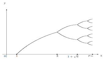
尽管逻辑斯蒂映射的迭代过程在参数经过一个又一个分叉点后看上去愈来愈复杂,但是如上所述,当
μ
n
−
1
<
μ
≤
μ
n
\mu_{n - 1} < \mu \leq \mu_n
μn−1<μ≤μn 时,对几乎所有的初始点,其迭代点列最终将收敛到那个吸引的周期 -
2
n
2^n
2n 轨道,因而迭代过程的最终性态还是可以预测的,这些都属于“有序”的范畴。
到目前为止,我们碰到的周期点的周期只是 1 和 2 的一些次方,而看不到周期为其他正整数的周期轨道。读者自然会问:当一个映射具有一个周期为 3 的点时,情况会怎么样?近半个世纪前马里兰大学的一位华人博士研究生李天岩(1945 - 2020)和他的博士论文导师约克(James Yorke, 1941 - )教授,在一篇著名文章《周期三则意味着混沌》(Period Three Implies Chaos)中,回答了这个问题,而且答案是令人惊奇的:
李 - 约克定理 设 S S S 是一个连续映射,将定义域区间映到自身。如果它有一个周期为 3 的点,则
- 对任一自然数 n n n, S S S 有一个周期为 n n n 的点。
- 存在定义域内的一个不可数的子集 A A A,它不包含周期点,使得对 A A A 中任意两个不同的点 x 0 x_0 x0 和 y 0 y_0 y0,分别从它们出发的对应迭代点的距离序列 ∣ S n ( x 0 ) − S n ( y 0 ) ∣ |S^n(x_0) - S^n(y_0)| ∣Sn(x0)−Sn(y0)∣ 当 n n n 趋于无穷大时,下极限为 0,而上极限大于 0。
- 对 A A A 中任一点 x 0 x_0 x0 及任一周期点 p p p,分别从它们出发的对应迭代点的距离序列 ∣ S n ( x 0 ) − S n ( p ) ∣ |S^n(x_0) - S^n(p)| ∣Sn(x0)−Sn(p)∣ 当 n n n 趋于无穷大时,上极限大于 0。
定理结论中的后两部分用到了数列的上、下极限概念,对这个概念不熟悉的读者可以这样直观地理解:在 n n n 趋于无穷大的过程中,分别与初始点 x 0 x_0 x0 和 y 0 y_0 y0 对应的迭代点 S n ( x 0 ) S^n(x_0) Sn(x0) 和 S n ( y 0 ) S^n(y_0) Sn(y0) 无穷多次地相互靠近(“吸引”),又无穷多次地相互离开(“排斥”)。李 - 约克定理说明,存在比所有的自然数还要多的初始点 x 0 x_0 x0,不仅由它们出发的迭代点列 { S n ( x 0 ) } \{S^n(x_0)\} {Sn(x0)} 不可能收敛,而且它们的最终性态也是不可预测的,其主要特征表现在迭代点列对于初始条件的敏感依赖性。
这种由周期 - 3 点的存在性而导致的确定性意义上的迭代点轨道不规则或“无序”的行为,足以让李天岩和约克在他们的文章中第一次定义了数学名词——混沌。这篇于 1975 年 12 月刊登在世界范围内读者人数最多的数学期刊《美国数学月刊》(The American Mathematical Monthly)上的八页短文,在普林斯顿高等研究院的物理学家戴森(Freeman Dyson, 1923 - 2020)于 2008 年为美国数学会该年度的“爱因斯坦讲座”而准备的演讲稿《鸟与蛙》(Birds and Frogs)中,被称为“数学文献中不朽的珍品之一。”这篇数学文章迄今已被引用了超过 5500 次,它的思想火花被六十年前“混沌之父”、麻省理工学院气象学教授洛伦茨(Edward Lorenz, 1917 - 2008)关于天气预报的那篇迄今引用次数超过 26500 次的文章《确定性的非周期流》(Deterministic Nonperiodic Flow)所点燃,可见部分伟大数学定理的来源根植于自然界的某些科学发现之中。
八、混沌映射的例子
我们举一个例子来帮助大家理解。最简单的非线性映射——帐篷映射 T T T,是这样被定义的:当 x x x 属于 [ 0 , 1 2 ] [0, \frac{1}{2}] [0,21] 时, T ( x ) = 2 x T(x) = 2x T(x)=2x,而当 x x x 属于 [ 1 2 , 1 ] [\frac{1}{2}, 1] [21,1] 时, T ( x ) = 2 ( 1 − x ) T(x) = 2(1 - x) T(x)=2(1−x)。它是一个逐段线性的函数。显而易见,它有一周期 - 3 轨道 2 7 , 4 7 , 6 7 \frac{2}{7}, \frac{4}{7}, \frac{6}{7} 72,74,76;见下图中的一个“回路”。
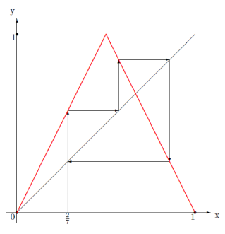
因而由李 - 约克定理知道帐篷映射是“李 - 约克混沌”的。事实上,对于 [ 0 , 1 ] [0, 1] [0,1] 中几乎所有的初始点 x 0 x_0 x0,其对应的迭代点列 { T n ( x 0 ) } \{T^n(x_0)\} {Tn(x0)} 在 [ 0 , 1 ] [0, 1] [0,1] 中稠密,即任给 [ 0 , 1 ] [0, 1] [0,1] 中的一个实数 x x x,存在 { T n ( x 0 ) } \{T^n(x_0)\} {Tn(x0)} 的一个子序列收敛到 x x x,因此这些迭代点好像如随机数那样在 [ 0 , 1 ] [0, 1] [0,1] 中跳来跳去,根本无法预测它们未来的走向。
另一个例子,通过一个类似矩阵相似变换那样所谓的“共轭变换”,我们可以找到当 μ \mu μ 取 4 时 S 4 ( x ) = 4 x ( 1 − x ) S_4(x) = 4x(1 - x) S4(x)=4x(1−x) 的一个周期 - 3 轨道
sin 2 ( π 7 ) , sin 2 ( 2 π 7 ) , sin 2 ( 4 π 7 ) \sin^2\left(\frac{\pi}{7}\right), \sin^2\left(\frac{2\pi}{7}\right), \sin^2\left(\frac{4\pi}{7}\right) sin2(7π),sin2(72π),sin2(74π)
所以它也是一个混沌映射。当自变量 x x x 限制在单位区间 [ 0 , 1 ] [0, 1] [0,1] 上,它的图像是在单位正方形 [ 0 , 1 ] 2 [0, 1]^2 [0,1]2 中“顶天立地”的抛物线:
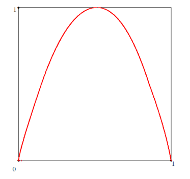
同样,对 [ 0 , 1 ] [0, 1] [0,1] 中几乎所有的初始点 x 0 x_0 x0,迭代点列 { ( S 4 ) n ( x 0 ) } \{(S_4)^n(x_0)\} {(S4)n(x0)} 在 [ 0 , 1 ] [0, 1] [0,1] 中处处稠密。然而,我们下面将知道,这些点列在区间中的分布方式和上面的帐篷映射完全不一样。
九、混沌映射的统计规律
总而言之,对于像帐篷映射 T T T 和逻辑斯蒂映射 S 4 S_4 S4 这样看似十分简单的非线性映射,对于几乎所有的迭代点列,其未来的最终走向是不可预测的。这是在“确定性意义”上的混沌,即当迭代的当前点知道后,下一个迭代点是由映射唯一所确定的,但从全局来看,迭代点又像随机数那样到处乱走,看上去似乎没有什么规律可循。由于这种迭代点的随机性并非来自像掷骰子那样的完全随机性,而是可以被认为是“局部确定性,长期随机性”,故此时混沌点列最终走向乱七八糟的状态也被称为“拟随机性”。
如上可见,对于混沌的映射,它的迭代点列的最终性态几乎是无法预测的,因而人们似乎对其长期行为难以琢磨,一筹莫展。是吗?对它们真的就找不到可循的规律吗?好的,现在让我们从另外一个角度来看混沌,也就是说,我们再从统计的观点来检视确定性意义上的混沌。
为了从统计的角度来观察混沌,我们再回到帐篷映射 T T T。让我们在定义域区间 [ 0 , 1 ] [0, 1] [0,1] 中取一个固定的子区间,比方说 [ 1 4 , 3 5 ] [\frac{1}{4}, \frac{3}{5}] [41,53]。在区间 [ 0 , 1 ] [0, 1] [0,1] 内随机地取一个初始点 x 0 x_0 x0,我们已经知道迭代点序列 { T n ( x 0 ) } \{T^n(x_0)\} {Tn(x0)} 在这个区间里如同随机数那样毫无章法地蹦来蹦去,但是我们来问一问下面这个问题:在这个迭代点列中的所有点中,跳进子区间 [ 1 4 , 3 5 ] [\frac{1}{4}, \frac{3}{5}] [41,53] 的频度是多少?或者说,在所有的迭代点中,那些进入 [ 1 4 , 3 5 ] [\frac{1}{4}, \frac{3}{5}] [41,53] 中的点所占的比例有多大?这是一个统计问题,或者说是一个概率问题。
在求解这个问题之前,我们指出帐篷映射的一个明显事实。给定 [ 0 , 1 ] [0, 1] [0,1] 的任意一个子区间 I I I,由下面的图示
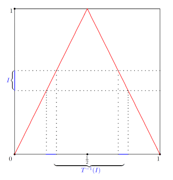
可见 I I I 的长度与它在帐篷映射下的逆像 T − 1 ( I ) T^{-1}(I) T−1(I)(两个有 I I I 的一半长度的子区间之并集)的长度一样。如果用专业一点的术语来说,作为区间长度概念之推广的“勒贝格测度”在帐篷映射下是一个“不变测度”,而帐篷映射是一个保持勒贝格测度不变的“保测变换”。换言之,对于 [ 0 , 1 ] [0, 1] [0,1] 的任意一个像模像样的子集(称为勒贝格可测子集),它的勒贝格测度等于它在帐篷映射下的逆像的勒贝格测度。法国数学家勒贝格(Henri Lebesgue, 1875 - 1941)于上个世纪初创立的“积分论”,是现代分析数学中不可或缺的基本工具。
十、伯克霍夫逐点遍历定理
要回答迭代点列 { T n ( x 0 ) } \{T^n(x_0)\} {Tn(x0)} 中的无穷多个点落到 [ 1 4 , 3 5 ] [\frac{1}{4}, \frac{3}{5}] [41,53] 的频度这个问题,我们先数一数,这个点列中的前 n n n 个点,即
x 0 , T ( x 0 ) , T 2 ( x 0 ) , … , T n − 1 ( x 0 ) x_0, T(x_0), T^2(x_0), \ldots, T^{n - 1}(x_0) x0,T(x0),T2(x0),…,Tn−1(x0)
中有多少个点进入 [ 1 4 , 3 5 ] [\frac{1}{4}, \frac{3}{5}] [41,53]。为了在数学上回答这个计数问题,我们引入一个集合 A A A 的“特征函数” χ A \chi_A χA 概念,它的定义是:若 x x x 属于 A A A,则 χ A ( x ) \chi_A(x) χA(x) 等于 1,若 x x x 不属于 A A A,则 χ A ( x ) \chi_A(x) χA(x) 等于 0。我们把在大学数学系的分析课程《实变函数论》中用来定义勒贝格积分第一步的这个特征函数,作为计数器用在这里。只要动动脑筋想一想,就会知道下面这个 n n n 个“非 0 即 1” 的数的和式 g
∑ k = 0 n − 1 χ A ( T k ( x 0 ) ) \sum_{k = 0}^{n - 1} \chi_A(T^k(x_0)) k=0∑n−1χA(Tk(x0))
恰恰表示前 n n n 个迭代点中进入 [ 1 4 , 3 5 ] [\frac{1}{4}, \frac{3}{5}] [41,53] 的那些点的个数。将这个非负整数再除以总的迭代点个数 n n n,即 g
1 n ∑ k = 0 n − 1 χ A ( T k ( x 0 ) ) \frac{1}{n} \sum_{k = 0}^{n - 1} \chi_A(T^k(x_0)) n1k=0∑n−1χA(Tk(x0))
就是 n n n 个迭代点中落到区间 [ 1 4 , 3 5 ] [\frac{1}{4}, \frac{3}{5}] [41,53] 的点的相对频度。我们的目的是求出整个无穷迭代点列中进入 [ 1 4 , 3 5 ] [\frac{1}{4}, \frac{3}{5}] [41,53] 的那些点的频度,很自然就必须取 n n n 趋于无穷大时上述相对频度的极限了。假如极限 g
lim n → ∞ 1 n ∑ k = 0 n − 1 χ A ( T k ( x 0 ) ) \lim_{n \to \infty} \frac{1}{n} \sum_{k = 0}^{n - 1} \chi_A(T^k(x_0)) n→∞limn1k=0∑n−1χA(Tk(x0))
存在,则这个极限值就是迭代点列 { T n ( x 0 ) } \{T^n(x_0)\} {Tn(x0)} 落到子区间 [ 1 4 , 3 5 ] [\frac{1}{4}, \frac{3}{5}] [41,53] 之中的频度或频率。它的更加专业的术语是 T T T 从初始点 x 0 x_0 x0 出发的迭代点列落到子区间 [ 1 4 , 3 5 ] [\frac{1}{4}, \frac{3}{5}] [41,53] 内的时间平均。
早在上世纪的 30 年代初,美国数学家伯克霍夫(George Birkhoff, 1884 - 1944)发表了遍历理论中的第一个遍历定理,现被称为“伯克霍夫逐点遍历定理”,有别于比它更早几个月用泛函分析方法证明出的“冯·诺伊曼平均遍历定理”。逐点遍历定理断言,如果一个关于某个概率测度的保测变换像帐篷映射 T T T 和逻辑斯蒂映射 S 4 S_4 S4 那样也是“遍历”的,即该变换具有某种意义上的“不可分解性”,则上述的频率或时间平均对几乎所有的初始点都存在,并且恰好等于所考虑子区间通过不变概率测度而算出来的概率测度值,称之为空间平均。由于区间 [ 0 , 1 ] [0, 1] [0,1] 上的勒贝格测度是帐篷映射的不变概率测度,而 [ 1 4 , 3 5 ] [\frac{1}{4}, \frac{3}{5}] [41,53] 的勒贝格测度值就是其长度 7 20 \frac{7}{20} 207,因此对几乎所有的初始点 x 0 x_0 x0,有 g
lim n → ∞ 1 n ∑ k = 0 n − 1 χ A ( T k ( x 0 ) ) = 7 20 \lim_{n \to \infty} \frac{1}{n} \sum_{k = 0}^{n - 1} \chi_A(T^k(x_0)) = \frac{7}{20} n→∞limn1k=0∑n−1χA(Tk(x0))=207
换言之,帐篷映射从几乎所有初始点 x 0 x_0 x0 出发的迭代点列 { T n ( x 0 ) } \{T^n(x_0)\} {Tn(x0)} 进入子区间 [ 1 4 , 3 5 ] [\frac{1}{4}, \frac{3}{5}] [41,53] 的频率,恰好等于同一个数——区间 [ 1 4 , 3 5 ] [\frac{1}{4}, \frac{3}{5}] [41,53] 的长度 7 20 \frac{7}{20} 207!
十一、帐篷映射的统计性质
这里有必要对伯克霍夫介绍两句。在他之前,美国名望最高的那几个数学家都是在欧洲几大科学圣地锻造成钢的,如他在芝加哥大学的博士论文导师穆尔(Eliakim Hastings Moore, 1862 - 1932)。伯克霍夫虽然是美国的“土博士”,日后却成了世界著名的数学家,而且一生执教于哈佛大学,并带动它的数学系脱胎换骨,成为美国乃至全球的数学研究重镇。他出道后的第一项大贡献是证明了庞加莱“最后的定理”,成为美国动力系统这一广泛领域的祖师爷。他的儿子长大后也出任哈佛的数学教授。
伯克霍夫逐点遍历定理关于帐篷映射的更一般结论是:任给定义域区间 [ 0 , 1 ] [0, 1] [0,1] 的一个勒贝格可测子集 A A A,对于 [ 0 , 1 ] [0, 1] [0,1] 中几乎所有的初始点 x 0 x_0 x0,都有
lim n → ∞ 1 n ∑ k = 0 n − 1 χ A ( T k ( x 0 ) ) = μ ( A ) \lim_{n \to \infty} \frac{1}{n} \sum_{k = 0}^{n - 1} \chi_A(T^k(x_0)) = \mu(A) n→∞limn1k=0∑n−1χA(Tk(x0))=μ(A)
其中 μ ( A ) \mu(A) μ(A) 是 A A A 的勒贝格测度。
这说明,尽管在确定性意义上帐篷映射是混沌的,具有对初始点的敏感依赖性,即初始点的微小变化导致迭代点列的可观变化,但在统计的意义上,对几乎所有的初始点,迭代点列进入定义域区间的任一“可测子集”的频率却是与初始点的选取无关的一个固定数,这个常数恰好等于所取子集的勒贝格测度。由此推出,对几乎所有的初始点,其迭代点列在 [ 0 , 1 ] [0, 1] [0,1] 上是一致分布的。
如上结论表明,在确定性意义上的混沌,在统计的意义上却可以失去“混沌”,而变得极有规律可循,这个规律数学上归功于伯克霍夫逐点遍历定理的发现。在物理上有类似的观察:就微观而言,单个分子的运动轨迹是紊乱无序的,但是在宏观的尺度上,大量分子的运动是有统计规律可循的,这就导致统计物理这门重要学科的诞生。事实上,冯·诺伊曼(John von Neumann, 1903 - 1957)和伯克霍夫等人所证明的第一代遍历定理,最初的动因就是来自于从数学上探讨统计物理中“玻尔兹曼遍历假设”是否具有合理性。
十二、逻辑斯蒂映射的统计性质
我们再看看另一个有名的混沌映射——逻辑斯蒂映射 S 4 ( x ) = 4 x ( 1 − x ) S_4(x) = 4x(1 - x) S4(x)=4x(1−x) 的情形。现在定义域区间 [ 0 , 1 ] [0, 1] [0,1] 中的子区间 I I I 的长度不再等于它在 S 4 S_4 S4 下的逆像 ( S 4 ) − 1 ( I ) (S_4)^{-1}(I) (S4)−1(I)(也是两个子区间的并集)的长度,换言之,勒贝格测度不再是 S 4 S_4 S4 的不变测度了。但是,如果我们定义一个新的“测度”,它将区间 [ a , b ] [a, b] [a,b] 的测度或“广义长度”定义为一个在 ( 0 , 1 ) (0, 1) (0,1) 上处处为正的函数
f ∗ ( x ) = 1 π x − x 2 f^*(x) = \frac{1}{\pi \sqrt{x - x^2}} f∗(x)=πx−x21
在 [ a , b ] [a, b] [a,b] 上的积分值,记为 μ f ∗ ( [ a , b ] ) \mu_{f^*}([a, b]) μf∗([a,b])。函数 f ∗ f^* f∗ 表达式分母中有 π \pi π 是为了保证它在 [ 0 , 1 ] [0, 1] [0,1] 上的积分等于 1,使得它成为一个密度函数。由于上述概率测度 μ f ∗ \mu_{f^*} μf∗ 是由密度函数 f ∗ f^* f∗ 所定义的,我们说它是绝对连续的。动一下手算一下积分,就可以简单地证明逻辑斯蒂映射保持这个概率测度不变,即
μ f ∗ ( ( S 4 ) − 1 ( [ a , b ] ) ) = μ f ∗ ( [ a , b ] ) \mu_{f^*}((S_4)^{-1}([a, b])) = \mu_{f^*}([a, b]) μf∗((S4)−1([a,b]))=μf∗([a,b])
对 [ 0 , 1 ] [0, 1] [0,1] 的所有子区间 [ a , b ] [a, b] [a,b] 都成立。这样,伯克霍夫逐点遍历定理告诉我们,逻辑斯蒂映射从几乎所有初始点 x 0 x_0 x0 出发的迭代点列 { ( S 4 ) n ( x 0 ) } \{(S_4)^n(x_0)\} {(S4)n(x0)} 进入子区间 [ a , b ] [a, b] [a,b] 的频率,等于 [ a , b ] [a, b] [a,b] 的新测度值:
lim n → ∞ 1 n ∑ k = 0 n − 1 χ [ a , b ] ( ( S 4 ) k ( x 0 ) ) = ∫ a b 1 π x − x 2 d x \lim_{n \to \infty} \frac{1}{n} \sum_{k = 0}^{n - 1} \chi_{[a, b]}((S_4)^k(x_0)) = \int_a^b \frac{1}{\pi \sqrt{x - x^2}} dx n→∞limn1k=0∑n−1χ[a,b]((S4)k(x0))=∫abπx−x21dx
由于上面这个密度函数的图像是像对称悬链线那样“向上弯曲”的,其结果是如果 [ 0 , 1 ] [0, 1] [0,1] 中的两个小区间具有一样的通常长度,但它们中的一个靠近 [ 0 , 1 ] [0, 1] [0,1] 的某个端点,另一个却靠近中间,则位于靠近边缘的那个子区间上方、被函数 1 π x − x 2 \frac{1}{\pi \sqrt{x - x^2}} πx−x21 的图像压住的曲边矩形有大一点的面积,也就是说它有较大一点的 μ f ∗ \mu_{f^*} μf∗ 测度值,如下图所示:
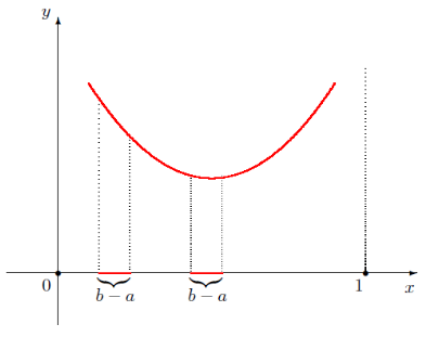
因而迭代点列落到这个子区间的频率比落到另一个子区间的频率要大。这实际上表明迭代点的序列在 [ 0 , 1 ] [0, 1] [0,1] 上不是一致分布的。由此可见,帐篷映射 T T T 与逻辑斯蒂映射 S 4 S_4 S4 在确定性意义上虽然都是混沌的,但它们各自的迭代点分布方式却是不一样的。它们分别按照某一个“概率密度函数”而在 [ 0 , 1 ] [0, 1] [0,1] 上分布,前者以常数函数 1 的方式均匀分布,而后者则由无界的密度函数 1 π x − x 2 \frac{1}{\pi \sqrt{x - x^2}} πx−x21 确定其迭代点列在定义域上的分布。
十三、弗罗贝尼乌斯 - 佩隆算子
决定逻辑斯蒂映射迭代点列分布规律的这个特别的密度函数 f ∗ f^* f∗,早在 1947 年就被美国“氢弹之父”乌拉姆(Stanislaw Ulam, 1909 - 1984)和“电子计算机之父”冯·诺伊曼发现了。现在的问题是,任意给出一个将 [ 0 , 1 ] [0, 1] [0,1] 映到自身的混沌映射 S S S,我们怎样去寻找一个在 S S S 下不变并且是绝对连续的概率测度呢?换言之,怎样找到一个密度函数 f ∗ f^* f∗,它所定义的绝对连续概率测度
μ f ∗ ( [ a , b ] ) = ∫ [ a , b ] f ∗ ( x ) d x \mu_{f^*}([a, b]) = \int_{[a, b]} f^*(x) dx μf∗([a,b])=∫[a,b]f∗(x)dx
是 S S S 的不变概率测度?如果找到了它,这个混沌映射的迭代点序列 { S n ( x 0 ) } \{S^n(x_0)\} {Sn(x0)} 在定义域区间上的统计分布规律就会借助于伯克霍夫逐点遍历定理而得到。
对这个问题的回答,需要一个以两个德国人名字命名的算子:弗罗贝尼乌斯 - 佩隆算子。其实弗罗贝尼乌斯(Georg Frobenius, 1849 - 1917)和佩隆(Oskar Perron, 1880 - 1975)这两人与该算子并无多大的关系,完全是因为他们的名气太响,以至于后人给他们再添名气,就像解非线性方程组著名的“牛顿法”名字也是“张冠李戴”所致。但是这个算子被如此命名还是有些道理的,因为在一百多年前,先是由年轻的佩隆(1907 年)然后由资深的弗罗贝尼乌斯(1912 年)分别对正矩阵和更广的不可约非负矩阵证明了他们的谱定理,主要内容之一为谱半径是特征值。这一套理论现以“非负矩阵的佩隆 - 弗罗贝尼乌斯理论”冠名,而这里提及的无穷维线性正算子和非负矩阵共享不少良好的性质,这就给予乌拉姆足够的理由在他的不朽著作《数学问题集》(A Collection of Mathematical Problems)中慷慨地借用了他们俩的大名。弗罗贝尼乌斯 - 佩隆算子的正式定义需要测度论知识,但我们可以用一个人人都懂的简单例子来描绘这个算子的基本思想。
假设两个物理系的教授张三和李四及数学系的一位教授王五申请某项研究基金,他们各自成功的概率分别为 1 2 \frac{1}{2} 21, 1 3 \frac{1}{3} 31 和 1 6 \frac{1}{6} 61。试问物理系和数学系获得该基金的概率为多少?
这个问题连小学生都能解答,但是我们为了说明问题,故意用“高射炮打蚊子”的方式来求解。定义一个映射 S S S,它把张教授和李教授映到物理系,把王教授映到数学系。在映射 S S S 的定义域 { \{ { 张教授,李教授,王教授 } \} } 上已经给出了一个概率分布 { 1 2 , 1 3 , 1 6 } \{ \frac{1}{2}, \frac{1}{3}, \frac{1}{6} \} {21,31,61},而通过 S S S 可将其定义域上的如上概率分布很自然地转移到其值域 { \{ { 物理系,数学系 } \} } 上,即子集 { \{ { 物理系 } \} } 的概率是它在 S S S 下的逆像 { \{ { 张教授,李教授 } \} } 的概率 1 2 + 1 3 = 5 6 \frac{1}{2} + \frac{1}{3} = \frac{5}{6} 21+31=65,而子集 { \{ { 数学系 } \} } 的概率是它在 S S S 下的逆像 { \{ { 王教授 } \} } 的概率 1 6 \frac{1}{6} 61。将定义域上的概率分布通过映射 S S S 转移到值域上的概率分布的这一依从关系,被称之为 S S S 所对应的弗罗贝尼乌斯 - 佩隆算子,记为 P S P_S PS。
我们把上面转移概率分布的思想用于一个混沌映射
S : [ 0 , 1 ] → [ 0 , 1 ] S \colon [0, 1] \to [0, 1] S:[0,1]→[0,1]
任给定义域上的一个概率测度 μ \mu μ,对于 [ 0 , 1 ] [0, 1] [0,1] 中的每一个子区间 I I I,我们将它在 S S S 下的逆像 S − 1 ( I ) S^{-1}(I) S−1(I) 的概率测度值 μ ( S − 1 ( I ) ) \mu(S^{-1}(I)) μ(S−1(I)) 转移到它身上来,即 I I I 的新的概率测度值等于 S − 1 ( I ) S^{-1}(I) S−1(I) 的旧的概率测度值。这种将概率分布 μ \mu μ 变为把 μ \mu μ 与逆像运算 S − 1 S^{-1} S−1 复合而成的概率分布的变换,称为对应于映射 S S S 的弗罗贝尼乌斯 - 佩隆算子 P S P_S PS。当概率分布 μ \mu μ 由密度函数 f f f 所定义,即 I I I 的测度值 μ ( I ) = ∫ I f ( x ) d x \mu(I) = \int_I f(x) dx μ(I)=∫If(x)dx 时,在所论映射是“非奇异”的假设下, μ \mu μ 与逆像运算 S − 1 S^{-1} S−1 复合而成的测度由一个记为 P S f P_S f PSf 的密度函数确定,这个密度函数满足下面的等式
∫ I P S f ( x ) d x = ∫ I ∗ f ( x ) d x \int_I P_S f(x) dx = \int_{I^*} f(x) dx ∫IPSf(x)dx=∫I∗f(x)dx
其中 I ∗ = S − 1 ( I ) I^* = S^{-1}(I) I∗=S−1(I)。由于上式对所有的子区间 I I I 都应该成立,我们可以取 I = [ 0 , x ] I = [0, x] I=[0,x],故有
∫ [ 0 , x ] P S f ( t ) d t = ∫ I ∗ f ( t ) d t \int_{[0, x]} P_S f(t) dt = \int_{I^*} f(t) dt ∫[0,x]PSf(t)dt=∫I∗f(t)dt
其中 I ∗ = S − 1 ( [ 0 , x ] ) I^* = S^{-1}([0, x]) I∗=S−1([0,x])。两边对变量 x x x 求导数,再利用微积分基本定理,就得到弗罗贝尼乌斯 - 佩隆算子的显式表达式
P
S
f
(
x
)
=
D
x
∫
I
∗
f
(
t
)
d
t
,
I
∗
=
S
−
1
(
[
0
,
x
]
)
P_S f(x) =D_x \int_{I^*} f(t) dt, \;I^* = S^{-1}([0, x])
PSf(x)=Dx∫I∗f(t)dt,I∗=S−1([0,x])
其中
D
x
D_x
Dx 表示对自变量
x
x
x 求导运算。
十四、弗罗贝尼乌斯 - 佩隆算子的应用
我们算一算当 S S S 是逻辑斯蒂映射 4 x ( 1 − x ) 4x(1 - x) 4x(1−x) 时,其对应的弗罗贝尼乌斯 - 佩隆算子的表达式是什么样子的。通过下图的演示,
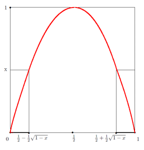
可以知道 [ 0 , x ] [0, x] [0,x] 在 S S S 下的逆像 S − 1 ( [ 0 , x ] ) S^{-1}([0, x]) S−1([0,x]) 是两个区间 [ 0 , 1 − 1 − x 2 ] [0, \frac{1 - \sqrt{1 - x}}{2}] [0,21−1−x] 和 [ 1 + 1 − x 2 , 1 ] [\frac{1 + \sqrt{1 - x}}{2}, 1] [21+1−x,1] 的并集,故由上述的公式得
P S f ( x ) = ( 1 − x ) − 1 / 2 4 { f ( 1 − 1 − x 2 ) + f ( 1 + 1 − x 2 ) } P_S f(x) = \frac{(1 - x)^{-1/2}}{4} \left\{ f\left( \frac{1 - \sqrt{1 - x}}{2} \right) + f\left( \frac{1 + \sqrt{1 - x}}{2} \right) \right\} PSf(x)=4(1−x)−1/2{f(21−1−x)+f(21+1−x)}
不难验证,密度函数 f ∗ ( x ) = 1 π x − x 2 f^*(x) = \frac{1}{\pi \sqrt{x - x^2}} f∗(x)=πx−x21 是上述算子的不动点,即 P S f ∗ ( x ) ≡ f ∗ ( x ) P_S f^*(x) \equiv f^*(x) PSf∗(x)≡f∗(x)。因为 f ∗ f^* f∗ 是 P S P_S PS 的不动点,我们也把它称为 P S P_S PS 的一个不变密度函数。它所定义的概率测度决定了混沌映射迭代点列的统计性质。
至于帐篷映射 T T T,因为 [ 0 , x ] [0, x] [0,x] 在 T T T 下的逆像 T − 1 ( [ 0 , x ] ) T^{-1}([0, x]) T−1([0,x]) 是两个区间 [ 0 , x 2 ] [0, \frac{x}{2}] [0,2x] 和 [ 1 − x 2 , 1 ] [1 - \frac{x}{2}, 1] [1−2x,1] 的并集,其对应的弗罗贝尼乌斯 - 佩隆算子有简单的表达式
P T f ( x ) = 1 2 { f ( x 2 ) + f ( 1 − x 2 ) } P_T f(x) = \frac{1}{2} \left\{ f\left( \frac{x}{2} \right) + f\left( 1 - \frac{x}{2} \right) \right\} PTf(x)=21{f(2x)+f(1−2x)}
显然,常数函数 f ∗ ( x ) ≡ 1 f^*(x) \equiv 1 f∗(x)≡1 是它的不变密度函数。这就解释了为何帐篷映射对几乎所有的初始点,其迭代点序列在 [ 0 , 1 ] [0, 1] [0,1] 上是一致分布的。
一般来说,确定性意义上的混沌映射,在统计的意义下常常具有正规的性态,它所对应的弗罗贝尼乌斯 - 佩隆算子的不变密度函数给出了混沌迭代点列的最终统计分布。从上世纪 70 年代初起,数学家们对不同类型的混沌映射所对应的弗罗贝尼乌斯 - 佩隆算子研究了不变密度函数的存在性,而另一方面,应用科学领域所需要的对数值求解这些不变密度函数的算法设计与收敛性分析,导致“计算遍历理论”这一当代学科的蓬勃发展。
十五、总结
如今,物理科学、工程科学和生命科学中的许多现象,都可以运用统计的观点进行研究而洞察其真相。这个观点不仅在统计物理这门重要学科中被发扬光大,而且导致了与人类福祉密切相关的几大新兴学科的兴起和发展,比方说无线通讯、搜索引擎、计算分子动力学及药物设计等。
这就是我们从统计的角度来察看混沌而观察到的一小片美景。
完稿于 2023 年 1 月 25 日星期三 美国哈蒂斯堡夏日山庄
via:
-
A brief history of chaos - appendHist.pdf
https://cns.gatech.edu/~predrag/courses/PHYS-7224-07/appendHist.pdf -
A history of chaos theory - PMC
https://pmc.ncbi.nlm.nih.gov/articles/PMC3202497/


 2743
2743

 被折叠的 条评论
为什么被折叠?
被折叠的 条评论
为什么被折叠?
 到【灌水乐园】发言


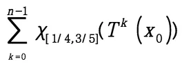
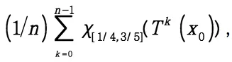
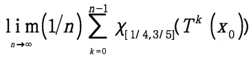
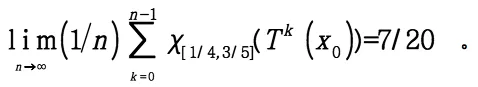