论文阅读-Non-intrusive load identification using reconstructed voltage–current images

Publisher: IEEE OPEN ACCESS

Date: MAY 2021

MOTIVATION OF READING: 在基于VI轨迹的方法中，不同的设备可能具有相同的轨迹

---

1. Overview 

Probelm statement: The identification of resistive appliances that have similar features in a power grid is still a major problem.

Methodology: the reconstructed image of a voltage-current (VI) trajectory is used as input
data for a convolutional neural network (CNN) to classify the appliances.

Validation: PLAID and IDOUC dataset. 

2. Relative Work

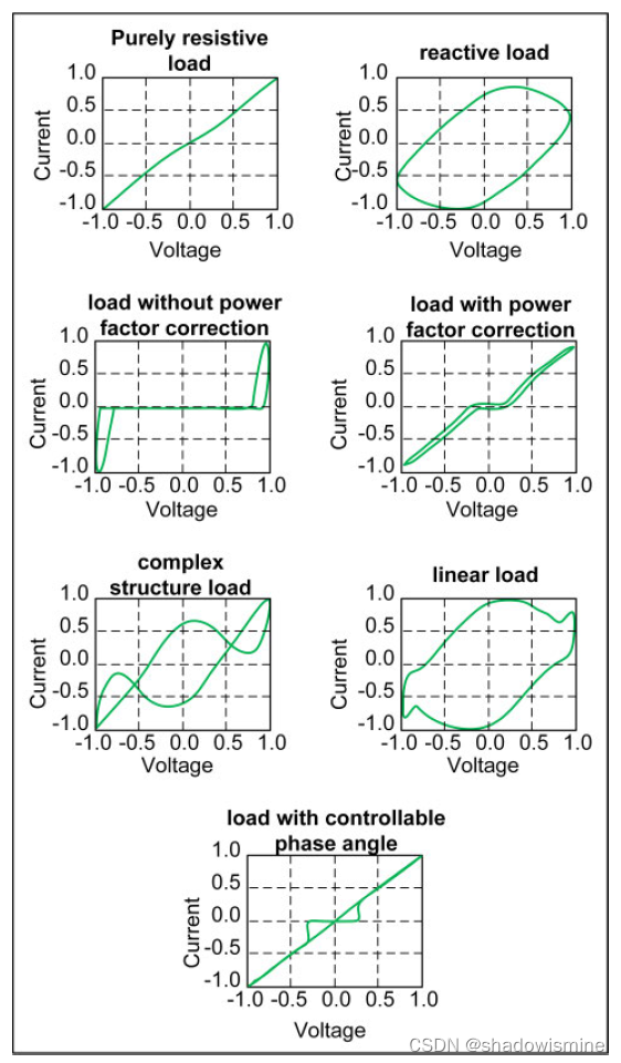
Liang et.al. [16] divide household appliances into 7 basic types, purely resistive load, reactive load, load without power factor correction, load with power factor correction, complex structure load, and linear load. The current trajectories of electric appliances of the same type are similar.

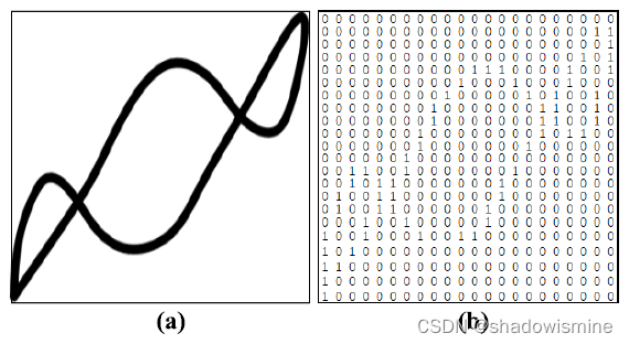
D. Liang et.al. proposed a method of constructing VI trajectory mapping by voltage and current data that extracted from the same single cycle, to identify different load types which is called binary VI trajectory mapping. 

This use of voltage and current cycle data to establish spatial relationships has a good load characteristic description ability. When the sampling rate of the electrical signal is high, and the picture used to generate the V-I trajectory mapping is small, it is easy to cause the loss of the high sampling rate data information details, and even cause the loss of some effective data features.

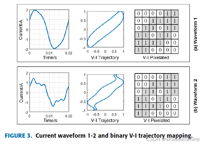
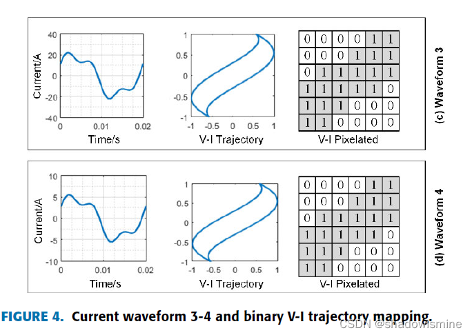
In Fig. 3, the current trajectories of waveform1 and waveform 2 are different. However, theirs binary VI trajectory mappings are the same. In Fig. 4, the peak current of waveform 3 is
about 22A, and the peak current of waveform 4 is about 6A.

3. Reconstruction Process

The specific construction process of the reconstructed VI trajectory graph is as follows:

1. The original voltage V and current I are measured when the appliance is in a steady-state and is active for a certain duration;

2. Several cycles for the voltage and the current are extracted individually according to the following condition: v(k) * v(k-1) < 0 U v(k-1) < 0;

3. The VI image is built;

4. the obtained VI image is then reconstructed by setting random thresholds for both the voltage and current using the equations below: (不是很看得懂)

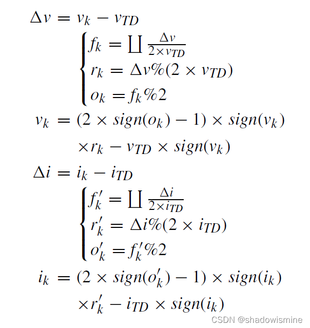
5. The reconstructed VI image should be normalized such that [V, I ] between -1 to 1.

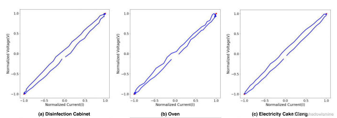
Original VI image:

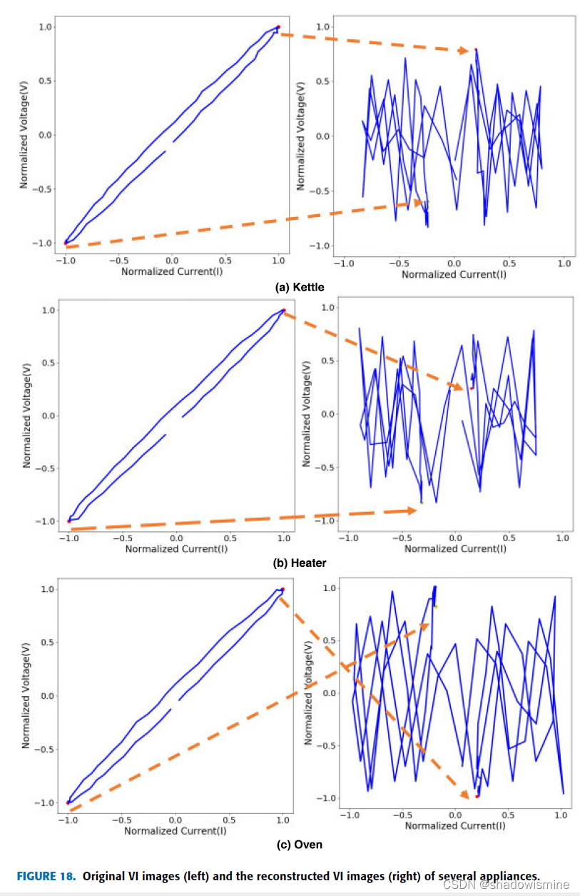
Reconstructed VI images:

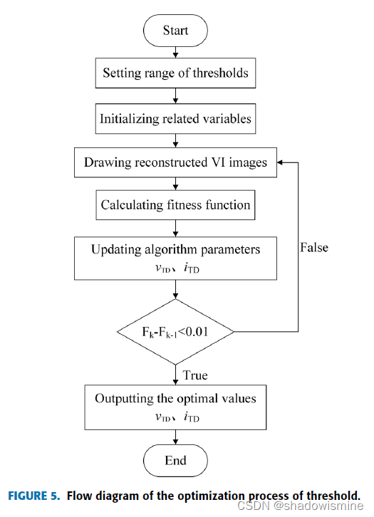
4. Threshold Optimization Based on PSO

An essential process for appliance identification is to set an optimal thresholds. The differences among the appliances can then be amplified. In this study, the particle swarm optimization (PSO) is used to search the optimal values of voltage and current.

5. Classification model based on CNN

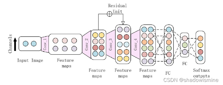
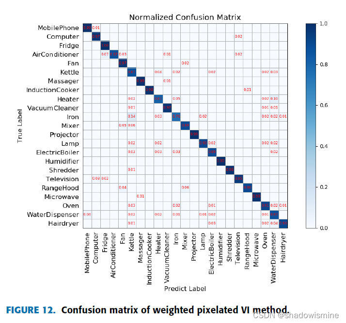
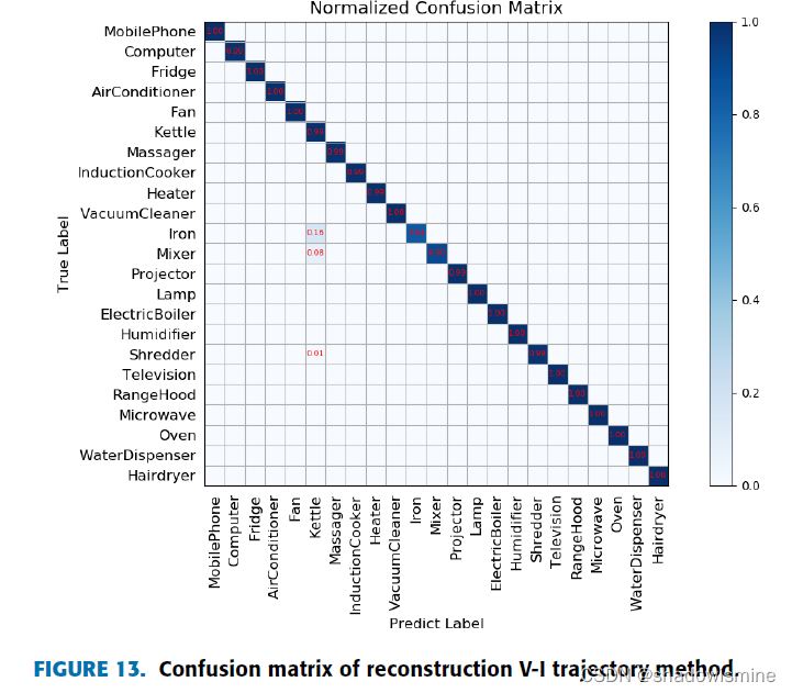
6. Experiment and Results

Two datasets called PLAID and OUCSEI. PLAID are used in this study to verify the proposed method.