集成学习实战之 -- RandomForest

一、引入

1.Linear model

∀ i ∈ { 1 , . . . , N } , y ^ i = ∑ j = 1 D w j X i j \forall_i\in{ \lbrace1,...,N\rbrace},\hat{y}_i=\sum^{D}_{j=1}w_jX_{ij} ∀i​∈{1,...,N},y^​i​=j=1∑D​wj​Xij​

矩阵形式：
$$\hat{\mathbf{y}}=\mathbf{X}\mathbf{w}$$

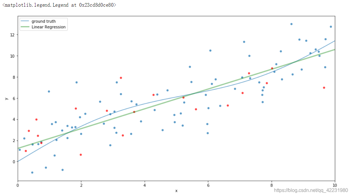
a.用线性模型拟合非线性数据：

1)拟合较平滑的曲线

FIGSIZE = (15,8)
def ground_truth(x):
    '''function to approximate'''
    return x + 2 * np.sin(0.1*x) + np.sin(0.6*x)
def gen_data(n_samples=200):
    '''产生训练和测试数据'''
    np.random.seed(42)
    X = np.random.uniform(0,10,size=n_samples)[:, np.newaxis]
    y = ground_truth(X.ravel()) + np.random.normal(scale=2,size=n_samples)
    
    X_train, X_test, y_train, y_test = train_test_split(X, y, test_size=0.2, random_state = 3)
    return X_train, X_test, y_train, y_test

def plot_data(alpha=0.7, s=20):
    fig = plt.figure(figsize=FIGSIZE)
    gt = plt.plot(x_plot, ground_truth(x_plot), alpha=alpha, label='ground truth')
    
    plt.scatter(X_train, y_train, s=s, alpha=alpha)
    plt.scatter(X_test, y_test, s=s, alpha=alpha, c='r')
    plt.xlim((0,10))
    plt.ylabel('y')
    plt.xlabel('x')

X_train, X_test, y_train, y_test = gen_data(100)
x_plot = np.linspace(0, 10, 500)

plot_data()

# 导入线性模型
est = LinearRegression().fit(X_train, y_train)
x_pred_1 = est.predict(x_plot[:,np.newaxis])
plt.plot(x_plot, x_pred_1, label='Linear Regression', c='g', alpha=0.4, linewidth=3)
plt.legend(loc='upper left')

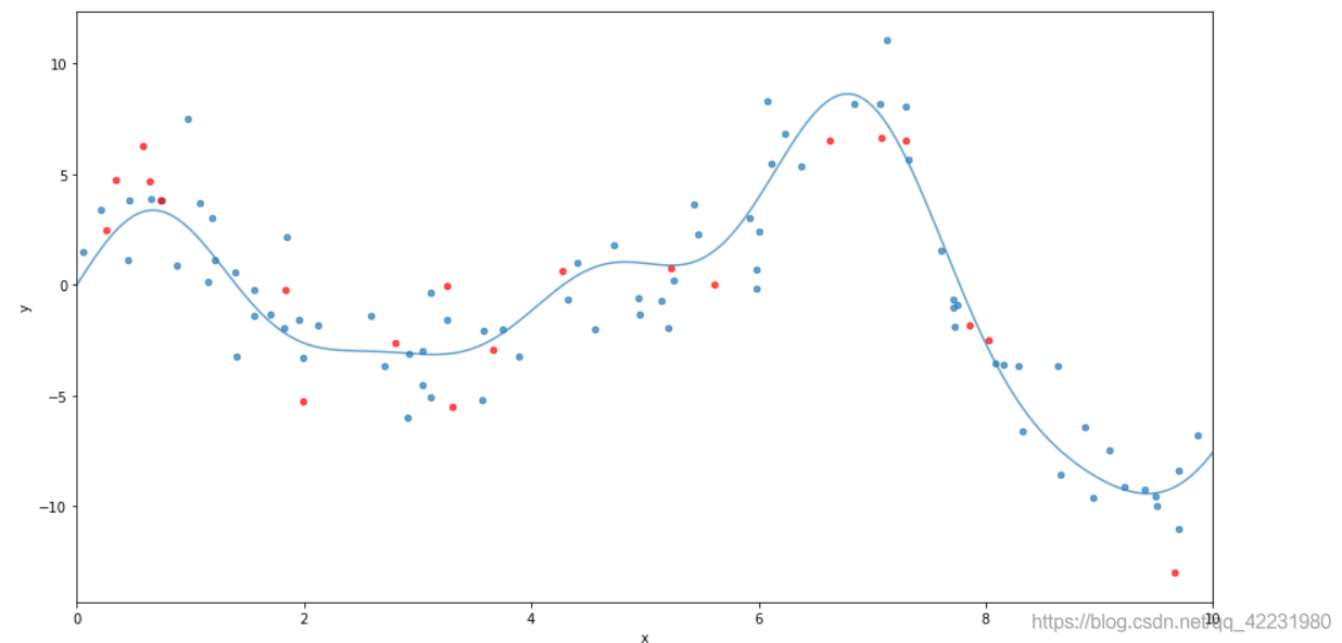
2）拟合不规则曲线

FIGSIZE = (15,8)
def ground_truth(x):
    '''function to approximate'''
    return x * np.cos(x) + 2 * np.sin(2*x) + np.sin(3*x)
def gen_data(n_samples=200):
    '''产生训练和测试数据'''
    np.random.seed(42)
    X = np.random.uniform(0,10,size=n_samples)[:, np.newaxis]
    y = ground_truth(X.ravel()) + np.random.normal(scale=2,size=n_samples)
    
    X_train, X_test, y_train, y_test = train_test_split(X, y, test_size=0.2, random_state = 3)
    return X_train, X_test, y_train, y_test

def plot_data(alpha=0.7, s=20):
    fig = plt.figure(figsize=FIGSIZE)
    gt = plt.plot(x_plot, ground_truth(x_plot), alpha=alpha, label='ground truth')
    
    plt.scatter(X_train, y_train, s=s, alpha=alpha)
    plt.scatter(X_test, y_test, s=s, alpha=alpha, c='r')
    plt.xlim((0,10))
    plt.ylabel('y')
    plt.xlabel('x')

X_train, X_test, y_train, y_test = gen_data(100)
x_plot = np.linspace(0, 10, 500)

plot_data()

plot_data()
est = LinearRegression().fit(X_train, y_train)
x_pred_1 = est.predict(x_plot[:,np.newaxis])
plt.plot(x_plot, x_pred_1, label='Linear Regression', c='r', alpha=0.4, linewidth=3)
plt.legend(loc='upper left')

此时再用线性拟合，效果非常的不好：

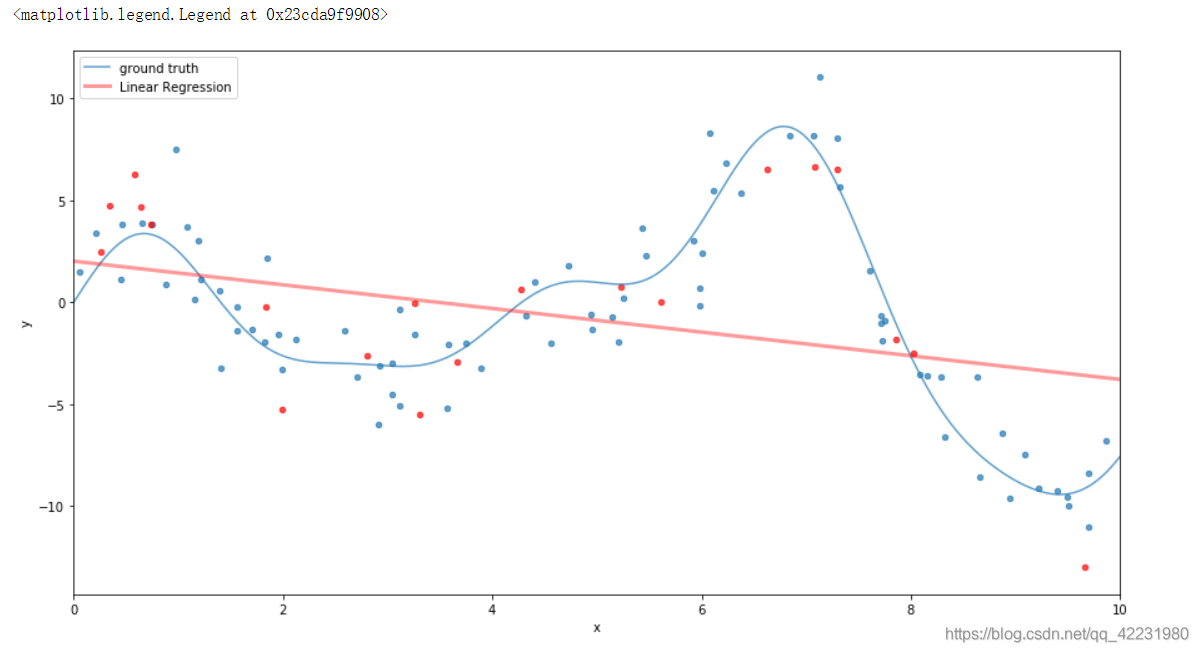
从图中可以看出，线性模型非常努力去贴合，但线性模型容量有限，不能拟合非线性的数据。

2.引入决策树

a.两个问题

1）决策树是线性模型吗？

• 一般都是非线性模型。

2）决策树能解决上面的问题吗？

后面给出答案。

b.决策树的特点

优点：

• 易解释(用了哪些特征去分离数据，阈值是多少，甚至可以手动写出一套规则)
• 原生支持特征选择
• 无需归一化
• 训练快

缺点：

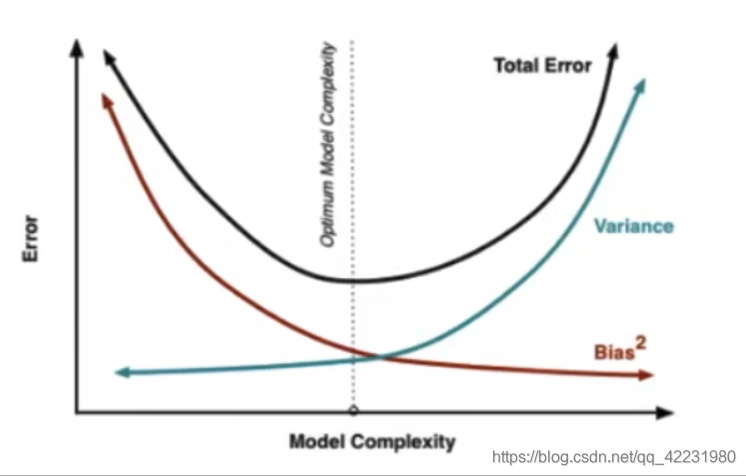
• low bias, high variance
• 不稳定，error propagation（每一次决策依赖上一次）
  可以参考：决策树实战
  

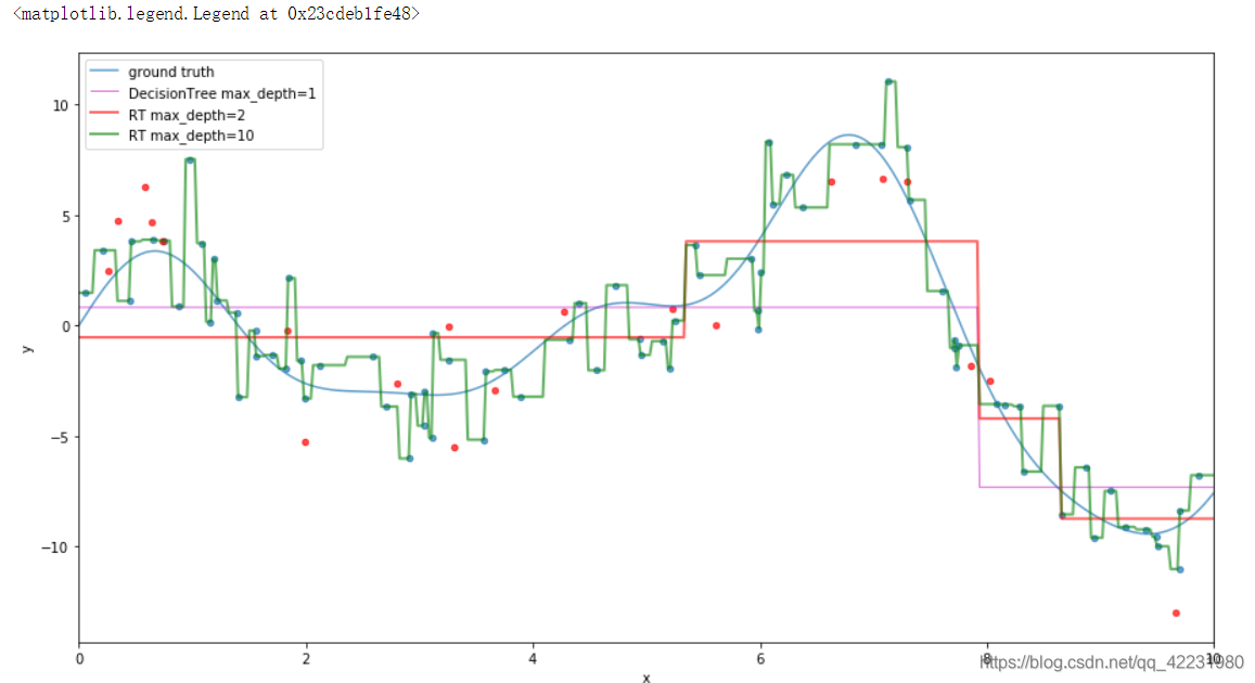
c.拟合数据

plot_data()
# 设置最大深度，分类一次
est = DecisionTreeRegressor(max_depth=1).fit(X_train, y_train)
x_pred_1 = est.predict(x_plot[:, np.newaxis])

plt.plot(x_plot, x_pred_1, label='DecisionTree max_depth=1',c='m', alpha=0.6, lw=1)

#随着深度的增加，单颗决策树在训练集上的准确率增加
est = DecisionTreeRegressor(max_depth=2).fit(X_train, y_train)
plt.plot(x_plot, est.predict(x_plot[:, np.newaxis]),
         label='RT max_depth=2', alpha=0.6, c='r', lw=2)
# 但深度一直增加会让训练集完全拟合，出现过拟合，使泛化能力变差
est = DecisionTreeRegressor(max_depth=20).fit(X_train, y_train)
plt.plot(x_plot, est.predict(x_plot[:, np.newaxis]),
         label='RT max_depth=10', alpha=0.6, c='g', lw=2)
plt.legend(loc='upper left')

二、模型融合

1.Bagging

现在可以回答“决策树能解决上面的问题吗？”，不完全能，因为决策树的缺点：依赖于上一次的决策，方差大容易过拟合。
减少方差的办法：Bagging，在训练集不同的随机抽取，构成 $M$个子训练集，每个训练集分别训练一棵树 $f_m(x)$
然后构成一个集成模型：
$$f(x)=\sum _{m=1}^M\frac{1}{M}{f}_m(x)$$

2.Random Forest

简单的Bagging导致训练出来的子模型高度相关，甚至是一样的模型，导致集成后的模型方差仍然很大。
解决：除了训练集随机构造，feature也随机选择一部分训练,这就是Random forest。

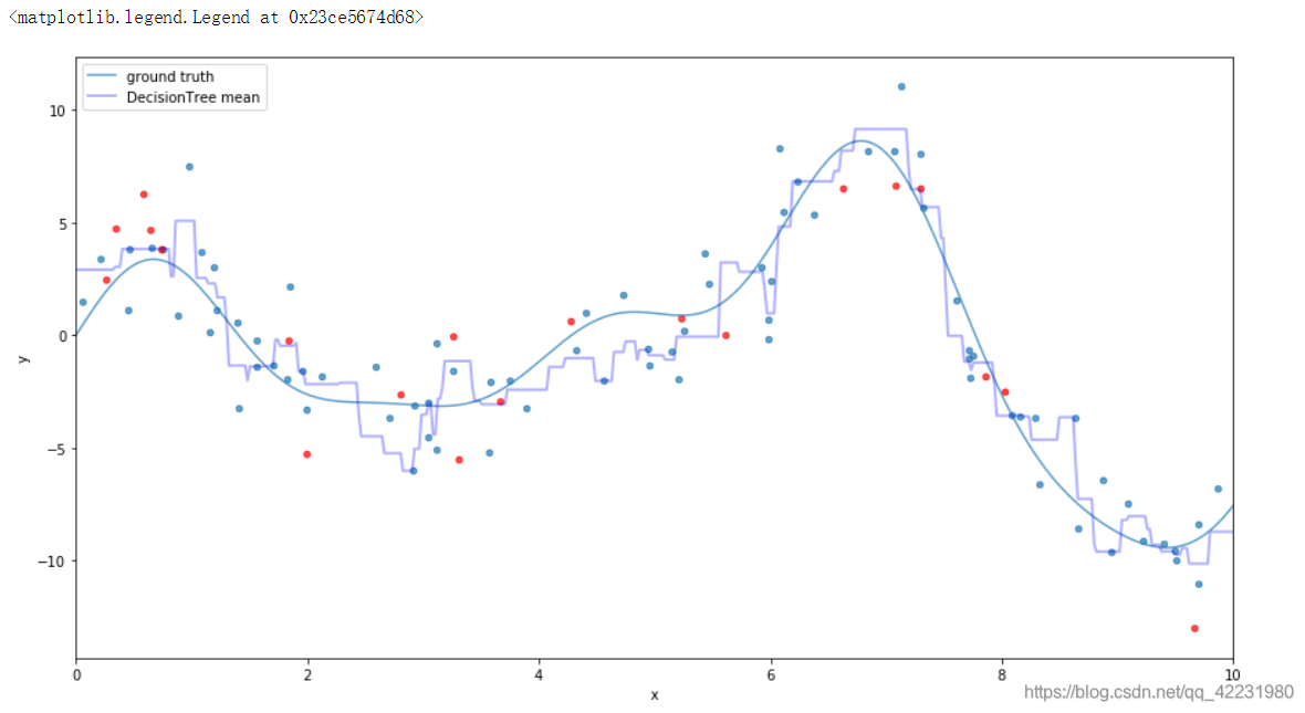
a.手动构建

plot_data()

col_sample = 0.6

seed_1 = np.random.RandomState(4)
# 随机采样80%
idx_1 = seed_1.randint(X_train.shape[0], size=int(col_sample*X_train.shape[0]))
# 当树的深度为20时，与上面对比，因为抽样80%所以并未完全拟合（蓝色的点）。
est = DecisionTreeRegressor(max_depth=20).fit(X_train[idx_1], y_train[idx_1])
x_pred_1 = est.predict(x_plot[:, np.newaxis])
# plt.plot(x_plot, x_pred_1, label='DecisionTree max_depth=1', c='g', alpha=0.5, lw=1)

# 对比：随机采样所以拟合的点不一样
idx_2 = seed_1.randint(X_train.shape[0], size=int(col_sample*X_train.shape[0]))
est = DecisionTreeRegressor(max_depth=20).fit(X_train[idx_2], y_train[idx_2])
x_pred_2 = est.predict(x_plot[:, np.newaxis])
# plt.plot(x_plot, x_pred_2, label='DecisionTree max_depth=2', c='r', alpha=0.5, lw=1)

# 
idx_3 = seed_1.randint(X_train.shape[0], size=int(col_sample*X_train.shape[0]))
est = DecisionTreeRegressor(max_depth=20).fit(X_train[idx_3], y_train[idx_3])
x_pred_3 = est.predict(x_plot[:, np.newaxis])
# plt.plot(x_plot, x_pred_3, label='DecisionTree max_depth=3', c='m', alpha=0.4, lw=1)

# 求均值，减缓过拟合（Bagging的思想）
x_pred_mean = np.mean([x_pred_1, x_pred_2, x_pred_3], axis=0)
plt.plot(x_plot, x_pred_mean, label='DecisionTree mean', c='b', alpha=0.3, lw=2)
plt.legend(loc='upper left')

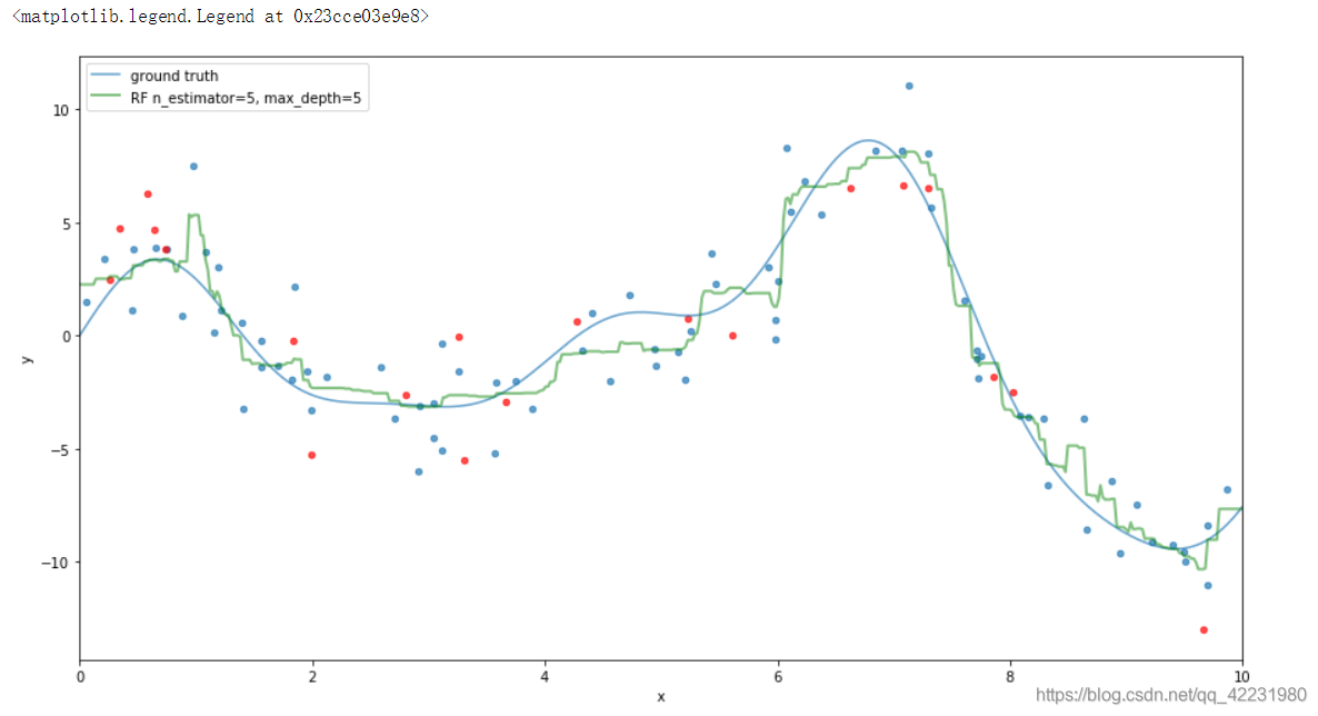
a.用sklearn中的模型构建

plot_data()

# est = RandomForestRegressor(n_estimators=10, max_depth=3).fit(X_train, y_train)
# plt.plot(x_plot, est.predict(x_plot[:, newaxis]),
#          label='RF n_estimator=10, max_depth=3', c='g',alpha=0.9,lw=2)

# est = RandomForestRegressor(n_estimators=100, max_depth=5).fit(X_train, y_train)
# plt.plot(x_plot, est.predict(x_plot[:, newaxis]),
#          label='RF n_estimator=100, max_depth=5', c='g',alpha=0.7,lw=2)
# 
est = RandomForestRegressor(n_estimators=100, max_depth=5).fit(X_train, y_train)
plt.plot(x_plot, est.predict(x_plot[:, newaxis]),
         label='RF n_estimator=5, max_depth=5', c='g',alpha=0.5,lw=2)

plt.legend(loc='upper left')