MATLAB实战：人工大猩猩部队GTO优化共振稀疏分解RSSD超参数

机器鱼

已于 2025-04-22 22:54:18 修改

阅读量1.5k

点赞数 1

分类专栏： Matlab神经网络1000个案例分析文章标签：优化算法

于 2022-11-10 08:14:38 首次发布

本文链接：https://blog.youkuaiyun.com/qq_41043389/article/details/127781659

版权

Matlab神经网络1000个案例分析专栏收录该内容

27 篇文章

订阅专栏

本文介绍了一种改进的共振稀疏分解方法，通过人工大猩猩部队优化算法（GTO）优化超参数，以减少受主观因素影响。研究者针对轴承振动信号，利用最小化相关峭度作为适应度函数，实现了更稳定的分解效果。最终优化了Q1, Q2, A1, A2和mu参数，提升了机械故障诊断的准确性。

摘要生成于 C知道，由 DeepSeek-R1 满血版支持，前往体验 >

本博客来源于优快云机器鱼，未同意任何人转载。

更多内容，欢迎点击本专栏目录，查看更多内容。

0.引言

共振稀疏分解是振动信号中脉冲成分提取的方法。与基于频率的信号处理方法不同，该方法同时参考频率和带宽两个因素，从而在分离信号不同成分的过程中能够很好处理信号不同成分的重叠问题。然而共振稀疏分解的分解效果受到品质因子 Q 、权重系数 A 以及拉格朗日乘子mu的主观选择影响。

为此，针对共振稀疏分解RSSD在振动信号分解过程中，分解效果受到多参数随机选择影响的缺陷，提出基于人工大猩猩部队优化算法的共振稀疏分解超参数优化算法，运用最小化相关峭度指标来作为适应度函数。

1.原理

1.1 共振稀疏分解

共振稀疏分解是最新提出的信号处理方法，不同于传统的基于频率或尺寸的信号处理方法，该方法在实现振动信号特征提取的过程中同时考虑信号的频率和带宽两因素，依据品质因子的不同，将振动信号的组成成分理解为周期谐波、故障冲击以及噪声三部分并分别分离到高低共振分量以及残余分量中。详细原理可以参看4中参考文献中的文献内容，这里只做简单叙述。需要用到tqwt_matlab_toolbox，该工具箱是用来做rssd分解的，这里是下载链接。

1.2 人工大猩猩部队优化算法

GTO是2021年新推出的智能优化算法，选择这个算法的目的就是比较新，目前用的人相对较少，详细原理戳这里。具体代码如下：


function [Silverback_Score,Silverback,convergence_curve]=GTO(pop_size,max_iter,lower_bound,upper_bound,variables_no,fobj)


% initialize Silverback
Silverback=[];
Silverback_Score=inf;

%Initialize the first random population of Gorilla
X=initialization(pop_size,variables_no,upper_bound,lower_bound);


convergence_curve=zeros(max_iter,1);

for i=1:pop_size
    Pop_Fit(i)=fobj(X(i,:));%#ok
    if Pop_Fit(i)<Silverback_Score
        Silverback_Score=Pop_Fit(i);
        Silverback=X(i,:);
    end
end


GX=X(:,:);
lb=ones(1,variables_no).*lower_bound;
ub=ones(1,variables_no).*upper_bound;

%%  Controlling parameter

p=0.03;
Beta=3;
w=0.8;

%%Main loop
for It=1:max_iter

    a=(cos(2*rand)+1)*(1-It/max_iter);
    C=a*(2*rand-1);

    %% Exploration:

    for i=1:pop_size
        if rand<p
            GX(i,:) =(ub-lb)*rand+lb;
        else
            if rand>=0.5
                Z = unifrnd(-a,a,1,variables_no);
                H=Z.*X(i,:);
                GX(i,:)=(rand-a)*X(randi([1,pop_size]),:)+C.*H;
            else
                GX(i,:)=X(i,:)-C.*(C*(X(i,:)- GX(randi([1,pop_size]),:))+rand*(X(i,:)-GX(randi([1,pop_size]),:))); %ok ok

            end
        end
    end

    GX = boundaryCheck(GX, lower_bound, upper_bound);

    % Group formation operation
    for i=1:pop_size
        New_Fit= fobj(GX(i,:));
        if New_Fit<Pop_Fit(i)
            Pop_Fit(i)=New_Fit;
            X(i,:)=GX(i,:);
        end
        if New_Fit<Silverback_Score
            Silverback_Score=New_Fit;
            Silverback=GX(i,:);
        end
    end

    %% Exploitation:
    for i=1:pop_size
        if a>=w
            g=2^C;
            delta= (abs(mean(GX)).^g).^(1/g);
            GX(i,:)=C*delta.*(X(i,:)-Silverback)+X(i,:);
        else

            if rand>=0.5
                h=randn(1,variables_no);
            else
                h=randn(1,1);
            end
            r1=rand;
            GX(i,:)= Silverback-(Silverback*(2*r1-1)-X(i,:)*(2*r1-1)).*(Beta*h);

        end
    end

    GX = boundaryCheck(GX, lower_bound, upper_bound);

    % Group formation operation
    for i=1:pop_size
        New_Fit= fobj(GX(i,:));
        if New_Fit<Pop_Fit(i)
            Pop_Fit(i)=New_Fit;
            X(i,:)=GX(i,:);
        end
        if New_Fit<Silverback_Score
            Silverback_Score=New_Fit;
            Silverback=GX(i,:);
        end
    end

    convergence_curve(It)=Silverback_Score;

end
end

% This function initialize the first population of search agents
function Positions=initialization(SearchAgents_no,dim,ub,lb)

Boundary_no= size(ub,2); % numnber of boundaries

% If the boundaries of all variables are equal and user enter a signle
% number for both ub and lb
if Boundary_no==1
    Positions=rand(SearchAgents_no,dim).*(ub-lb)+lb;
end

% If each variable has a different lb and ub
if Boundary_no>1
    for i=1:dim
        ub_i=ub(i);
        lb_i=lb(i);
        Positions(:,i)=rand(SearchAgents_no,1).*(ub_i-lb_i)+lb_i;
    end
end
end

function  X  = boundaryCheck(X, lb, ub)

for i=1:size(X,1)
    FU=X(i,:)>ub;
    FL=X(i,:)<lb;
    X(i,:)=(X(i,:).*(~(FU+FL)))+ub.*FU+lb.*FL;
end
end

搭配上主函数即可运行，代码如下：

function []=main()
clear ;close all;clc;format compact
N=30; % Number of search agents
T=500; % Maximum number of iterations
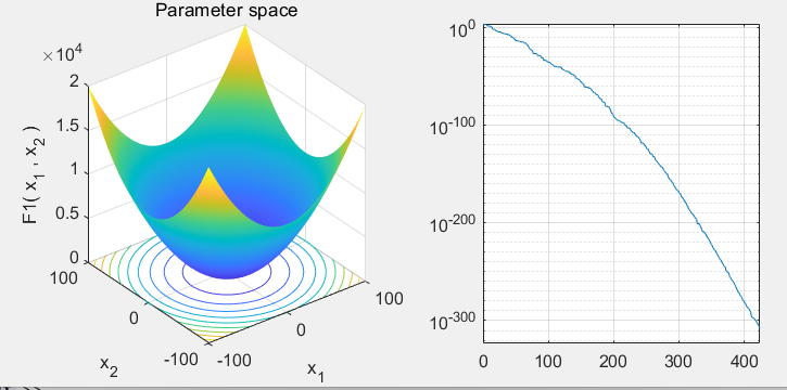
Function_name='F1'; % Name of the test function that can be from F1 to F23 (Table 1,2,3 in the paper) 设定适应度函数
[lb,ub,dim,fobj]=Get_Functions_details(Function_name);  %设定边界以及优化函数
[Destination_fitness,bestPositions,Convergence_curve]=GTO(N,T,lb,ub,dim,fobj);
figure('Position',[269   240   660   290])
subplot(1,2,1);
func_plot(Function_name);
title('Parameter space')
xlabel('x_1');
ylabel('x_2');
zlabel([Function_name,'( x_1 , x_2 )'])
subplot(1,2,2);
semilogy(Convergence_curve)
grid on
end


% This function draw the benchmark functions

function func_plot(func_name)

[lb,ub,dim,fobj]=Get_Functions_details(func_name);

switch func_name
    case 'F1'
        x=-100:2:100; y=x; %[-100,100]

    case 'F2'
        x=-100:2:100; y=x; %[-10,10]

    case 'F3'
        x=-100:2:100; y=x; %[-100,100]

    case 'F4'
        x=-100:2:100; y=x; %[-100,100]
    case 'F5'
        x=-200:2:200; y=x; %[-5,5]
    case 'F6'
        x=-100:2:100; y=x; %[-100,100]
    case 'F7'
        x=-1:0.03:1;  y=x  %[-1,1]
    case 'F8'
        x=-500:10:500;y=x; %[-500,500]
    case 'F9'
        x=-5:0.1:5;   y=x; %[-5,5]
    case 'F10'
        x=-20:0.5:20; y=x;%[-500,500]
    case 'F11'
        x=-500:10:500; y=x;%[-0.5,0.5]
    case 'F12'
        x=-10:0.1:10; y=x;%[-pi,pi]
    case 'F13'
        x=-5:0.08:5; y=x;%[-3,1]
    case 'F14'
        x=-100:2:100; y=x;%[-100,100]
    case 'F15'
        x=-5:0.1:5; y=x;%[-5,5]
    case 'F16'
        x=-1:0.01:1; y=x;%[-5,5]
    case 'F17'
        x=-5:0.1:5; y=x;%[-5,5]
    case 'F18'
        x=-5:0.06:5; y=x;%[-5,5]
    case 'F19'
        x=-5:0.1:5; y=x;%[-5,5]
    case 'F20'
        x=-5:0.1:5; y=x;%[-5,5]
    case 'F21'
        x=-5:0.1:5; y=x;%[-5,5]
    case 'F22'
        x=-5:0.1:5; y=x;%[-5,5]
    case 'F23'
        x=-5:0.1:5; y=x;%[-5,5]
end



L=length(x);
f=[];

for i=1:L
    for j=1:L
        if strcmp(func_name,'F15')==0 && strcmp(func_name,'F19')==0 && strcmp(func_name,'F20')==0 && strcmp(func_name,'F21')==0 && strcmp(func_name,'F22')==0 && strcmp(func_name,'F23')==0
            f(i,j)=fobj([x(i),y(j)]);
        end
        if strcmp(func_name,'F15')==1
            f(i,j)=fobj([x(i),y(j),0,0]);
        end
        if strcmp(func_name,'F19')==1
            f(i,j)=fobj([x(i),y(j),0]);
        end
        if strcmp(func_name,'F20')==1
            f(i,j)=fobj([x(i),y(j),0,0,0,0]);
        end
        if strcmp(func_name,'F21')==1 || strcmp(func_name,'F22')==1 ||strcmp(func_name,'F23')==1
            f(i,j)=fobj([x(i),y(j),0,0]);
        end
    end
end

surfc(x,y,f,'LineStyle','none');

end

% This function containts full information and implementations of the benchmark
% lb is the lower bound: lb=[lb_1,lb_2,...,lb_d]
% up is the uppper bound: ub=[ub_1,ub_2,...,ub_d]
% dim is the number of variables (dimension of the problem)

function [lb,ub,dim,fobj] = Get_Functions_details(F)


switch F
    case 'F1'
        fobj = @F1;
        lb=-100;
        ub=100;
        dim=30;

    case 'F2'
        fobj = @F2;
        lb=-10;
        ub=10;
        dim=30;

    case 'F3'
        fobj = @F3;
        lb=-100;
        ub=100;
        dim=30;

    case 'F4'
        fobj = @F4;
        lb=-100;
        ub=100;
        dim=30;

    case 'F5'
        fobj = @F5;
        lb=-30;
        ub=30;
        dim=30;

    case 'F6'
        fobj = @F6;
        lb=-100;
        ub=100;
        dim=30;

    case 'F7'
        fobj = @F7;
        lb=-1.28;
        ub=1.28;
        dim=30;

    case 'F8'
        fobj = @F8;
        lb=-500;
        ub=500;
        dim=30;

    case 'F9'
        fobj = @F9;
        lb=-5.12;
        ub=5.12;
        dim=30;

    case 'F10'
        fobj = @F10;
        lb=-32;
        ub=32;
        dim=30;

    case 'F11'
        fobj = @F11;
        lb=-600;
        ub=600;
        dim=30;

    case 'F12'
        fobj = @F12;
        lb=-50;
        ub=50;
        dim=30;

    case 'F13'
        fobj = @F13;
        lb=-50;
        ub=50;
        dim=30;

    case 'F14'
        fobj = @F14;
        lb=-65.536;
        ub=65.536;
        dim=2;

    case 'F15'
        fobj = @F15;
        lb=-5;
        ub=5;
        dim=4;

    case 'F16'
        fobj = @F16;
        lb=-5;
        ub=5;
        dim=2;

    case 'F17'
        fobj = @F17;
        lb=[-5,0];
        ub=[10,15];
        dim=2;

    case 'F18'
        fobj = @F18;
        lb=-2;
        ub=2;
        dim=2;

    case 'F19'
        fobj = @F19;
        lb=0;
        ub=1;
        dim=3;

    case 'F20'
        fobj = @F20;
        lb=0;
        ub=1;
        dim=6;

    case 'F21'
        fobj = @F21;
        lb=0;
        ub=10;
        dim=4;

    case 'F22'
        fobj = @F22;
        lb=0;
        ub=10;
        dim=4;

    case 'F23'
        fobj = @F23;
        lb=0;
        ub=10;
        dim=4;
end

end

% F1

function o = F1(x)
o=sum(x.^2);
end

% F2

function o = F2(x)
o=sum(abs(x))+prod(abs(x));
end

% F3

function o = F3(x)
dim=size(x,2);
o=0;
for i=1:dim
    o=o+sum(x(1:i))^2;
end
end

% F4

function o = F4(x)
o=max(abs(x));
end

% F5

function o = F5(x)
dim=size(x,2);
o=sum(100*(x(2:dim)-(x(1:dim-1).^2)).^2+(x(1:dim-1)-1).^2);
end

% F6

function o = F6(x)
o=sum(abs((x+.5)).^2);
end

% F7

function o = F7(x)
dim=size(x,2);
o=sum([1:dim].*(x.^4))+rand;
end

% F8

function o = F8(x)
o=sum(-x.*sin(sqrt(abs(x))));
end

% F9

function o = F9(x)
dim=size(x,2);
o=sum(x.^2-10*cos(2*pi.*x))+10*dim;
end

% F10

function o = F10(x)
dim=size(x,2);
o=-20*exp(-.2*sqrt(sum(x.^2)/dim))-exp(sum(cos(2*pi.*x))/dim)+20+exp(1);
end

% F11

function o = F11(x)
dim=size(x,2);
o=sum(x.^2)/4000-prod(cos(x./sqrt([1:dim])))+1;
end

% F12

function o = F12(x)
dim=size(x,2);
o=(pi/dim)*(10*((sin(pi*(1+(x(1)+1)/4)))^2)+sum((((x(1:dim-1)+1)./4).^2).*...
    (1+10.*((sin(pi.*(1+(x(2:dim)+1)./4)))).^2))+((x(dim)+1)/4)^2)+sum(Ufun(x,10,100,4));
end

% F13

function o = F13(x)
dim=size(x,2);
o=.1*((sin(3*pi*x(1)))^2+sum((x(1:dim-1)-1).^2.*(1+(sin(3.*pi.*x(2:dim))).^2))+...
    ((x(dim)-1)^2)*(1+(sin(2*pi*x(dim)))^2))+sum(Ufun(x,5,100,4));
end

% F14

function o = F14(x)
aS=[-32 -16 0 16 32 -32 -16 0 16 32 -32 -16 0 16 32 -32 -16 0 16 32 -32 -16 0 16 32;,...
    -32 -32 -32 -32 -32 -16 -16 -16 -16 -16 0 0 0 0 0 16 16 16 16 16 32 32 32 32 32];

for j=1:25
    bS(j)=sum((x'-aS(:,j)).^6);
end
o=(1/500+sum(1./([1:25]+bS))).^(-1);
end

% F15

function o = F15(x)
aK=[.1957 .1947 .1735 .16 .0844 .0627 .0456 .0342 .0323 .0235 .0246];
bK=[.25 .5 1 2 4 6 8 10 12 14 16];bK=1./bK;
o=sum((aK-((x(1).*(bK.^2+x(2).*bK))./(bK.^2+x(3).*bK+x(4)))).^2);
end

% F16

function o = F16(x)
o=4*(x(1)^2)-2.1*(x(1)^4)+(x(1)^6)/3+x(1)*x(2)-4*(x(2)^2)+4*(x(2)^4);
end

% F17

function o = F17(x)
o=(x(2)-(x(1)^2)*5.1/(4*(pi^2))+5/pi*x(1)-6)^2+10*(1-1/(8*pi))*cos(x(1))+10;
end

% F18

function o = F18(x)
o=(1+(x(1)+x(2)+1)^2*(19-14*x(1)+3*(x(1)^2)-14*x(2)+6*x(1)*x(2)+3*x(2)^2))*...
    (30+(2*x(1)-3*x(2))^2*(18-32*x(1)+12*(x(1)^2)+48*x(2)-36*x(1)*x(2)+27*(x(2)^2)));
end

% F19

function o = F19(x)
aH=[3 10 30;.1 10 35;3 10 30;.1 10 35];cH=[1 1.2 3 3.2];
pH=[.3689 .117 .2673;.4699 .4387 .747;.1091 .8732 .5547;.03815 .5743 .8828];
o=0;
for i=1:4
    o=o-cH(i)*exp(-(sum(aH(i,:).*((x-pH(i,:)).^2))));
end
end

% F20

function o = F20(x)
aH=[10 3 17 3.5 1.7 8;.05 10 17 .1 8 14;3 3.5 1.7 10 17 8;17 8 .05 10 .1 14];
cH=[1 1.2 3 3.2];
pH=[.1312 .1696 .5569 .0124 .8283 .5886;.2329 .4135 .8307 .3736 .1004 .9991;...
    .2348 .1415 .3522 .2883 .3047 .6650;.4047 .8828 .8732 .5743 .1091 .0381];
o=0;
for i=1:4
    o=o-cH(i)*exp(-(sum(aH(i,:).*((x-pH(i,:)).^2))));
end
end

% F21

function o = F21(x)
aSH=[4 4 4 4;1 1 1 1;8 8 8 8;6 6 6 6;3 7 3 7;2 9 2 9;5 5 3 3;8 1 8 1;6 2 6 2;7 3.6 7 3.6];
cSH=[.1 .2 .2 .4 .4 .6 .3 .7 .5 .5];

o=0;
for i=1:5
    o=o-((x-aSH(i,:))*(x-aSH(i,:))'+cSH(i))^(-1);
end
end

% F22

function o = F22(x)
aSH=[4 4 4 4;1 1 1 1;8 8 8 8;6 6 6 6;3 7 3 7;2 9 2 9;5 5 3 3;8 1 8 1;6 2 6 2;7 3.6 7 3.6];
cSH=[.1 .2 .2 .4 .4 .6 .3 .7 .5 .5];

o=0;
for i=1:7
    o=o-((x-aSH(i,:))*(x-aSH(i,:))'+cSH(i))^(-1);
end
end

% F23

function o = F23(x)
aSH=[4 4 4 4;1 1 1 1;8 8 8 8;6 6 6 6;3 7 3 7;2 9 2 9;5 5 3 3;8 1 8 1;6 2 6 2;7 3.6 7 3.6];
cSH=[.1 .2 .2 .4 .4 .6 .3 .7 .5 .5];

o=0;
for i=1:10
    o=o-((x-aSH(i,:))*(x-aSH(i,:))'+cSH(i))^(-1);
end
end

function o=Ufun(x,a,k,m)
o=k.*((x-a).^m).*(x>a)+k.*((-x-a).^m).*(x<(-a));
end

2 GTO优化共振稀疏分解参数

2.1 数据准备

采用的是凯斯西储大学的故障轴承数据，这里【下载】,其时域图如下：

2.2 RSSD分解

直接设置参数进行RSSD分解，代码如下：

clc;clear;close all
addpath(genpath('tqwt_matlab_toolbox/'))
%% 加载数据
load 130.mat
b=X130_DE_time';
fs=12000;
N = 1024;
signal = b(1:N);%信号
t = (0:N-1)/fs;
%% 参数设置
Q1 = 9.51; A1=0.9;r1 = 3.5; J1 = 31; % High Q-factor TQWT
Q2 = 1.13; A2=0.1;r2 = 3.5; J2 = 11; % Low Q-factor TQWT
mu = 2.0; % SALSA parameter
Nit = 20; % Number of iterations
%% rssd分解
now1 = ComputeNow(N,Q1,r1,J1,'radix2'); % Compute norms of wavelets
now2 = ComputeNow(N,Q2,r2,J2,'radix2'); % Compute norms of wavelets

lam1 = A1*now1; % Regularization params for high Q-factor TQWT
lam2 = A2*now2; % Regularization params for low Q-factor TQWT

[x1,x2,w1s,w2s,costfn]=dualQd(signal,Q1,r1,J1,Q2,r2,J2,lam1,lam2,mu,Nit);%对信号进行共振稀疏分解
x1;%高共振分量
x2;%低共振分量
r=signal - x1 - x2;%残余量
%% 画图
figure
plot(t,signal);%显示原始信号
title('原始信号');
xlabel('时间t/s');
ylabel('幅值A');
box off

figure
plot(t,x1);%显示高共振分量
box off
title('HIGH Q-FACTOR COMPONENT');
xlabel('时间t/s');
ylabel('幅值A');

figure
plot(t,x2);%显示低共振分量
box off
title('LOW Q-FACTOR COMPONENT')
xlabel('时间t/s');
ylabel('幅值A');

figure
plot(t, r);%显示冗余分量
box off
title('RESIDUAL')
xlabel('时间t/s');
ylabel('幅值A');

2.3 优化原理

看过我之前博客的同学都知道，任意一个智能优化算法我们拿来用，是不用管具体原理的，只需根据我们要优化的目标修改优化的参数数量、范围，以及攥写适应度函数即可，这篇博客也是这样，主要步骤如下：

步骤1：知道要优化的参数的优化范围。根据【基于粒子群优化的共振稀疏分解在轴承故障诊断中的应用】与【改进的共振稀疏分解方法及在机械故障诊断中的应用】，我们知道都是优化参数是Q1、Q2、A1、A2、mu这5个参数，我们给他设置的范围如下：分别是 Q1的范围是[3 20], Q2的范围是[1 3] ,A1和A2范围是[0 1]，mu的范围是[0 1]，这些范围读者是可以根据自己的第六感修改的。


function [Silverback_Score,Silverback,convergence_curve]=GTO(signal)

pop_size=10;%
max_iter=10;%迭代次数
variables_no=5;%寻优维度
%5个待优化参数 分别是 Q1的范围是[3 20], Q2的范围是[1 3] ,A1和A2范围是[0 1]，mu的范围是[0 1]
lower_bound=[3 1 0 0 0];
upper_bound=[20 3 1 1 1];%寻优上下界


% initialize Silverback
Silverback=[];
Silverback_Score=inf;

%Initialize the first random population of Gorilla
X=initialization(pop_size,variables_no,upper_bound,lower_bound);


convergence_curve=zeros(max_iter,1);

for i=1:pop_size
    Pop_Fit(i)=fobj(signal,X(i,:));%#ok
    if Pop_Fit(i)<Silverback_Score
        Silverback_Score=Pop_Fit(i);
        Silverback=X(i,:);
    end
end


GX=X(:,:);
lb=ones(1,variables_no).*lower_bound;
ub=ones(1,variables_no).*upper_bound;

%%  Controlling parameter

p=0.03;
Beta=3;
w=0.8;

%%Main loop
for It=1:max_iter
    
    a=(cos(2*rand)+1)*(1-It/max_iter);
    C=a*(2*rand-1);
    
    %% Exploration:
    
    for i=1:pop_size
        if rand<p
            GX(i,:) =(ub-lb)*rand+lb;
        else
            if rand>=0.5
                Z = unifrnd(-a,a,1,variables_no);
                H=Z.*X(i,:);
                GX(i,:)=(rand-a)*X(randi([1,pop_size]),:)+C.*H;
            else
                GX(i,:)=X(i,:)-C.*(C*(X(i,:)- GX(randi([1,pop_size]),:))+rand*(X(i,:)-GX(randi([1,pop_size]),:))); %ok ok
                
            end
        end
    end
    
    GX = boundaryCheck(GX, lower_bound, upper_bound);
    
    % Group formation operation
    for i=1:pop_size
        New_Fit= fobj(signal,GX(i,:));
        if New_Fit<Pop_Fit(i)
            Pop_Fit(i)=New_Fit;
            X(i,:)=GX(i,:);
        end
        if New_Fit<Silverback_Score
            Silverback_Score=New_Fit;
            Silverback=GX(i,:);
        end
    end
    
    %% Exploitation:
    for i=1:pop_size
        if a>=w
            g=2^C;
            delta= (abs(mean(GX)).^g).^(1/g);
            GX(i,:)=C*delta.*(X(i,:)-Silverback)+X(i,:);
        else
            
            if rand>=0.5
                h=randn(1,variables_no);
            else
                h=randn(1,1);
            end
            r1=rand;
            GX(i,:)= Silverback-(Silverback*(2*r1-1)-X(i,:)*(2*r1-1)).*(Beta*h);
            
        end
    end
    
    GX = boundaryCheck(GX, lower_bound, upper_bound);
    
    % Group formation operation
    for i=1:pop_size
        New_Fit= fobj(signal,GX(i,:));
        if New_Fit<Pop_Fit(i)
            Pop_Fit(i)=New_Fit;
            X(i,:)=GX(i,:);
        end
        if New_Fit<Silverback_Score
            Silverback_Score=New_Fit;
            Silverback=GX(i,:);
        end
    end
    
    convergence_curve(It)=Silverback_Score;
    
end

% This function initialize the first population of search agents
function Positions=initialization(SearchAgents_no,dim,ub,lb)

Boundary_no= size(ub,2); % numnber of boundaries

% If the boundaries of all variables are equal and user enter a signle
% number for both ub and lb
if Boundary_no==1
    Positions=rand(SearchAgents_no,dim).*(ub-lb)+lb;
end

% If each variable has a different lb and ub
if Boundary_no>1
    for i=1:dim
        ub_i=ub(i);
        lb_i=lb(i);
        Positions(:,i)=rand(SearchAgents_no,1).*(ub_i-lb_i)+lb_i;
    end
end

function [ X ] = boundaryCheck(X, lb, ub)

    for i=1:size(X,1)
            FU=X(i,:)>ub;
            FL=X(i,:)<lb;
            X(i,:)=(X(i,:).*(~(FU+FL)))+ub.*FU+lb.*FL;
    end
end

步骤2：知道优化的目标。优化的目标是提高的RSSD分解准确率，所以我们的目标找到一种目标来评价怎么才知道RSSD更准，有了这个评价指标，我们就可以构建适应度函数，目的是通过GTO找到5个参数，用这5个参数构建RSSD分解的准确率最高。这一步需要查阅文献，参考文献中采用的是相关谱峭度，我们也用这个，主要是我也不知道用啥呀，我不是这个专业的。

步骤3：确定适应度函数，首先我们观察GTO的适应度曲线是一个下降的曲线，所以我们知道GTO是用来做最小化极值寻优的，因为我们的适应度函数也要越小代表找到的参数最优，文献中是最大化适应度函数K，而因为我们的算法是最小化极值寻优，因此我们最小化1/K，效果是一样的，代码如下：

function fit=fobj(s,pop)
%适应度函数，
%% 待优化的参数  --
% 基于粒子群优化的共振稀疏分解在轴承故障诊断中的应用与改进的共振稀疏分解方法及在机械故障诊断中的应用都是优化这5各参数
Q1=pop(1);
Q2=pop(2);
A1=pop(3);
A2=pop(4);
mu=pop(5);
%% 其余参数设置
r1 = 3.5; J1 = 31; % High Q-factor TQWT
r2 = 3.5; J2 = 11; % Low Q-factor TQWT
Nit = 20; % Number of iterations
N=length(s);
%% rssd分解
now1 = ComputeNow(N,Q1,r1,J1,'radix2'); % Compute norms of wavelets
now2 = ComputeNow(N,Q2,r2,J2,'radix2'); % Compute norms of wavelets

lam1 = A1*now1; % Regularization params for high Q-factor TQWT
lam2 = A2*now2; % Regularization params for low Q-factor TQWT

[x1,x2,~,~,~]=dualQd(s,Q1,r1,J1,Q2,r2,J2,lam1,lam2,mu,Nit);%对降噪后信号进行共振稀疏分解
% x1;%高共振分量
% x2;%低共振分量
% r=s - x1 - x2;%残余量

% 计算低共振分量x2的相关峭度
T=1/107.364; %基于奇异值分解和相关峭度的滚动轴承故障诊断方法研究说T=故障频率的倒数
M=6;
[k]=Correlated_Kurtosis(x2,T,M);
% 计算高低共振分量的相关系数
corrlation=(corr(x1',x2')+1)/2;%person的是[-1,1] 我们将其改成[0 1]
fit=k/corrlation;

end
function ckIter = Correlated_Kurtosis(x,T,M)
if( isempty(T) )
    T = 0;
end
if( isempty(M) )
    M = 1;
end

% Validate the inputs
if( sum( size(x) > 1 ) > 1 )
    error('Input signal x must be a 1d vector.')
elseif( sum(size(T) > 1) ~= 0 || T < 0 )
    error('Input argument T must be a zero or positive scalar.')
elseif( sum(size(M) > 1) ~= 0 || M < 1 || round(M)-M ~= 0 )
    error('Input argument M must be a positive integer scalar.')
end
% Force x into a column vector
x = x(:);
% Perform a resampling of x to an integer period if required
if( abs(round(T) - T) > 0.01 )
    % We need to resample x to an integer period
    T_new = ceil(T);
    % The rate transformation factor
    Factor = 20;
    
    % Calculate the resample factor
    P = round(T_new * Factor);
    Q = round(T * Factor);
    Common = gcd(P,Q);
    P = P / Common;
    Q = Q / Common;
    
    % Resample the input
    x = resample(x, P, Q);
    T = T_new;
else
    T = round(T);
end

N = length(x);
y=x;
% Generate yt
yt = zeros(N,M);
for( m = 0:M )
    if( m == 0 )
        yt(:,m+1) = y;
    else
        yt(T+1:end,m+1) = yt(1:end-T,m);
    end
end
% Calculate the ck value
ckIter = sum(prod(yt,2).^2)/( sum(y.^2)^(M+1) );

end

步骤4：构建调用这些原理的主函数

% 实现共振稀疏分解参数的优化
% 主要参考【改进的共振稀疏分解方法及在机械故障诊断中的应用】 
% 对Q1 Q2 A1 A2 mu这5个参数进行优化
clc;clear;close all;format compact
addpath(genpath('tqwt_matlab_toolbox/'))
tic
%% 加载分解的数据
load 130.mat
b = X130_DE_time';
N = 4096;% 信号长度
fs=12000;%采样频率
signal = b(1:N);%信号
t = (0:N-1)/fs;%时间间隔
%%
[~,pop,Convergence_curve]=GTO(signal);
%% 最优参数 
figure
plot(Convergence_curve)
title('适应度曲线')

disp('最优Q1 Q2 A1 A2 mu为：')
Q1=pop(1)
Q2=pop(2)
A1=pop(3)
A2=pop(4)
mu=pop(5)
%% 其余参数设置
r1 = 3.5; J1 = 31; % High Q-factor TQWT
r2 = 3.5; J2 = 11; % Low Q-factor TQWT
Nit = 20; % Number of iterations
N=length(signal);
%% rssd分解
now1 = ComputeNow(N,Q1,r1,J1,'radix2'); % Compute norms of wavelets
now2 = ComputeNow(N,Q2,r2,J2,'radix2'); % Compute norms of wavelets
lam1 = A1*now1; % Regularization params for high Q-factor TQWT
lam2 = A2*now2; % Regularization params for low Q-factor TQWT

[x1,x2,~,~,~]=dualQd(signal,Q1,r1,J1,Q2,r2,J2,lam1,lam2,mu,Nit);%对降噪后信号进行共振稀疏分解
% x1;%高共振分量
% x2;%低共振分量
r=signal - x1 - x2;%残余量
%% 画图
figure
plot(t,signal);%显示原始信号
title('原始信号');
xlabel('时间t/s');
ylabel('幅值A');
box off

figure
plot(t,x1);%显示高共振分量
box off
title('HIGH Q-FACTOR COMPONENT');
xlabel('时间t/s');
ylabel('幅值A');

figure
plot(t,x2);%显示低共振分量
box off
title('LOW Q-FACTOR COMPONENT')
xlabel('时间t/s');
ylabel('幅值A');

figure
plot(t, r);%显示冗余分量
box off
title('RESIDUAL')
xlabel('时间t/s');
ylabel('幅值A');

toc

由于我们是最小化适应度函数，所以适应度曲线是一条下降的曲线，如图

优化后的最优Q1 Q2 A1 A2 mu为：Q1 = 20；Q2 = 1.1104；A1 = 0.0274；A2 = 0.1262；
mu = 0.0081；