


环境准备
# 导入必要的库 / Import necessary libraries
import mujoco
import numpy as np
import matplotlib.pyplot as plt
from matplotlib.animation import FuncAnimation
import mediapy as media
from typing import List, Tuple, Optional, Dict
import time
from IPython.display import HTML

# 设置随机种子 / Set random seed
np.random.seed(42)
机械臂设计与建模
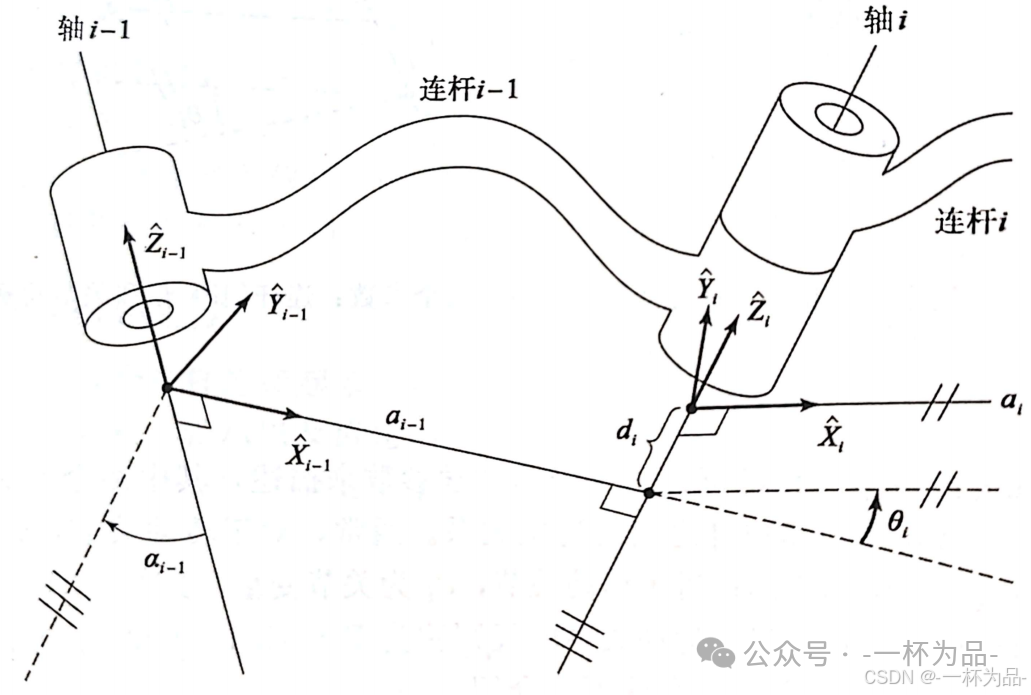
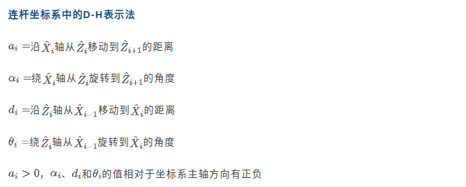
回顾【机器人学导论】Ep3.操作臂(正向)运动学,机械臂的设计参数由 D-H 表示法给出:
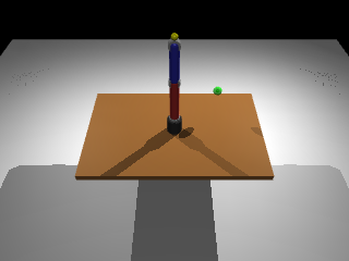
本节演示使用三自由度机械臂:
- 关节 1:基座旋转
- 关节 2:肩部俯仰
- 关节 3:肘部俯仰
在我们的简化模型中,两个连杆是位于同一平面的直杆,因此 α i \alpha_i αi 和 d i d_i di 均为 0(除了 α 0 = 9 0 ∘ \alpha_0=90^\circ α0=90∘),只需给出连杆长度 d i d_i di 即可。 θ i \theta_i θi 作为关节变量需配置其运动范围。
下面这个机械臂参数类除了运动学相关参数,还定义了一些外观参数:
# 定义机械臂参数 / Define arm parameters
class ArmParameters:
    """机械臂参数类 / Arm parameters class"""
    def __init__(self):
        # 连杆长度 / Link lengths
        self.base_height = 0.1
        self.link1_length = 0.3  # 上臂 / Upper arm
        self.link2_length = 0.25  # 前臂 / Forearm

        # 连杆半径 / Link radii
        self.base_radius = 0.05
        self.link_radius = 0.03

        # 关节限位 (度) / Joint limits (degrees)
        self.joint_limits = [
            (-180, 180),  # 基座旋转 / Base rotation
            (-90, 90),    # 肩部俯仰 / Shoulder pitch
            (-135, 135)   # 肘部俯仰 / Elbow pitch
        ]

        # 颜色 / Colors
        self.base_color = [0.2, 0.2, 0.2, 1]     # 深灰 / Dark gray
        self.link1_color = [0.8, 0.2, 0.2, 1]    # 红色 / Red
        self.link2_color = [0.2, 0.2, 0.8, 1]    # 蓝色 / Blue
        self.joint_color = [0.7, 0.7, 0.7, 1]    # 浅灰 / Light gray

params = ArmParameters()
def create_3dof_arm_xml(params: ArmParameters) -> str:
    """
    创建3自由度机械臂的MJCF XML / Create MJCF XML for 3-DOF arm
    """
    xml = f"""
    <mujoco model="3dof_robotic_arm">
        <!-- 仿真参数 / Simulation parameters -->
        <option timestep="0.001" gravity="0 0 -9.81" integrator="RK4"/>

        <!-- 默认设置 / Default settings -->
        <default>
            <joint armature="0.01" damping="0.1"/>
            <geom contype="1" conaffinity="1" friction="1 0.1 0.1" solref="0.02 1"/>
            <motor ctrllimited="true" ctrlrange="-1 1"/>
        </default>

        <!-- 资源 / Assets -->
        <asset>
            <material name="floor_mat" specular="0.3" shininess="0.1" rgba="0.8 0.8 0.8 1"/>
            <material name="base_mat" rgba="{' '.join(map(str, params.base_color))}"/>
            <material name="link1_mat" rgba="{' '.join(map(str, params.link1_color))}"/>
            <material name="link2_mat" rgba="{' '.join(map(str, params.link2_color))}"/>
            <material name="joint_mat" rgba="{' '.join(map(str, params.joint_color))}"/>
        </asset>

        <!-- 世界 / World -->
        <worldbody>
            <!-- 光源 / Lights -->
            <light name="light1" pos="2 2 2" dir="-1 -1 -1" diffuse="1 1 1"/>
            <light name="light2" pos="-2 2 2" dir="1 -1 -1" diffuse="0.5 0.5 0.5"/>

            <!-- 地面 / Ground -->
            <geom name="floor" type="plane" size="2 2 0.1" material="floor_mat"/>

            <!-- 工作台 / Workbench -->
            <body name="table" pos="0 0 0.4">
                <geom name="tabletop" type="box" size="0.6 0.4 0.02" rgba="0.6 0.4 0.2 1"/>
            </body>

            <!-- 机械臂基座 / Arm base -->
            <body name="base" pos="0 0 0.42">
                <geom name="base_geom" type="cylinder" size="{params.base_radius} {params.base_height}" material="base_mat"/>

                <!-- 关节1: 基座旋转 / Joint 1: Base rotation -->
                <body name="link1" pos="0 0 {params.base_height}">
                    <joint name="joint1" type="hinge" axis="0 0 1"
                           range="{params.joint_limits[0][0]} {params.joint_limits[0][1]}"/>
                    <geom name="joint1_geom" type="cylinder" size="{params.link_radius*1.2} 0.02" material="joint_mat"/>

                    <!-- 上臂 / Upper arm -->
                    <geom name="link1_geom" type="capsule"
                          fromto="0 0 0.02 0 0 {params.link1_length}"
                          size="{params.link_radius}" material="link1_mat"/>

                    <!-- 关节2: 肩部俯仰 / Joint 2: Shoulder pitch -->
                    <body name="link2" pos="0 0 {params.link1_length}">
                        <joint name="joint2" type="hinge" axis="0 1 0"
                               range="{params.joint_limits[1][0]} {params.joint_limits[1][1]}"/>
                        <geom name="joint2_geom" type="cylinder" size="{params.link_radius*1.2} 0.02" material="joint_mat" euler="90 0 0"/>

                        <!-- 前臂 / Forearm -->
                        <geom name="link2_geom" type="capsule"
                              fromto="0 0 0.02 0 0 {params.link2_length}"
                              size="{params.link_radius}" material="link2_mat"/>

                        <!-- 关节3: 肘部俯仰 / Joint 3: Elbow pitch -->
                        <body name="link3" pos="0 0 {params.link2_length}">
                            <joint name="joint3" type="hinge" axis="0 1 0"
                                   range="{params.joint_limits[2][0]} {params.joint_limits[2][1]}"/>
                            <geom name="joint3_geom" type="cylinder" size="{params.link_radius*1.2} 0.02" material="joint_mat" euler="90 0 0"/>

                            <!-- 末端执行器 / End effector -->
                            <body name="end_effector" pos="0 0 0.05">
                                <geom name="ee_geom" type="sphere" size="0.02" rgba="1 1 0 1"/>
                                <site name="ee_site" pos="0 0 0" size="0.01" rgba="1 0 0 1"/>
                            </body>
                        </body>
                    </body>
                </body>
            </body>

            <!-- 目标标记 / Target marker -->
            <body name="target" pos="0.3 0.2 0.6">
                <geom name="target_geom" type="sphere" size="0.03" rgba="0 1 0 0.5" contype="0" conaffinity="0"/>
                <site name="target_site" pos="0 0 0" size="0.01" rgba="0 1 0 1"/>
            </body>
        </worldbody>

        <!-- 执行器 / Actuators -->
        <actuator>
            <!-- 位置控制器 / Position controllers -->
            <position name="joint1_pos" joint="joint1" kp="100" ctrlrange="{params.joint_limits[0][0]} {params.joint_limits[0][1]}"/>
            <position name="joint2_pos" joint="joint2" kp="100" ctrlrange="{params.joint_limits[1][0]} {params.joint_limits[1][1]}"/>
            <position name="joint3_pos" joint="joint3" kp="100" ctrlrange="{params.joint_limits[2][0]} {params.joint_limits[2][1]}"/>

            <!-- 速度控制器 (备选) / Velocity controllers (alternative) -->
            <velocity name="joint1_vel" joint="joint1" kv="10"/>
            <velocity name="joint2_vel" joint="joint2" kv="10"/>
            <velocity name="joint3_vel" joint="joint3" kv="10"/>
        </actuator>

        <!-- 传感器 / Sensors -->
        <sensor>
            <!-- 关节位置传感器 / Joint position sensors -->
            <jointpos name="joint1_pos_sensor" joint="joint1"/>
            <jointpos name="joint2_pos_sensor" joint="joint2"/>
            <jointpos name="joint3_pos_sensor" joint="joint3"/>

            <!-- 关节速度传感器 / Joint velocity sensors -->
            <jointvel name="joint1_vel_sensor" joint="joint1"/>
            <jointvel name="joint2_vel_sensor" joint="joint2"/>
            <jointvel name="joint3_vel_sensor" joint="joint3"/>

            <!-- 末端执行器位置 / End effector position -->
            <framepos name="ee_pos" objtype="site" objname="ee_site"/>

            <!-- 目标距离 / Distance to target -->
            <rangefinder name="ee_target_dist" site="ee_site"/>
        </sensor>
    </mujoco>
    """
    return xml

# 创建模型 / Create model
arm_xml = create_3dof_arm_xml(params)
arm_model = mujoco.MjModel.from_xml_string(arm_xml)
arm_data = mujoco.MjData(arm_model)
正向运动学分析
回顾一下【机器人学导论】Ep3.操作比(正向)运动学的内容,对一个具有 n n n个自由度的操作臂来说,它的所有连杆位置可由一组 n n n个关节变量确定,这样的一组变量被称为 n × 1 n\times1 n×1的关节向量,所有关节向量组成的空间称为关节空间。将已知的关节空间描述转化为在笛卡尔空间中的描述,称为正向运动学,反之则为逆运动学。
一般情况下,正向运动学的计算需要根据连杆参数构成连杆变换矩阵。本例机械臂结构简单,且暂不考虑姿态问题,因此可直接求解:
def forward_kinematics(q: np.ndarray, params: ArmParameters) -> np.ndarray:
    """
    计算正向运动学 / Compute forward kinematics

    Args:
        q: 关节角度 [q1, q2, q3] (radians)
        params: 机械臂参数 / Arm parameters

    Returns:
        末端执行器位置 [x, y, z]
    """
    q1, q2, q3 = q

    # 基座高度 / Base height
    z0 = 0.42 + params.base_height

    # 计算各关节位置 / Calculate joint positions
    # 关节2位置 / Joint 2 position
    x2 = 0
    y2 = 0
    z2 = z0 + params.link1_length

    # 末端执行器位置 / End effector position
    # 考虑所有旋转 / Consider all rotations
    l2 = params.link2_length
    l3 = 0.05 # 包括末端大小 / Including end

    x = (l2 * np.sin(q2) + l3 * np.sin(q2 + q3)) * np.cos(q1)
    y = (l2 * np.sin(q2) + l3 * np.sin(q2 + q3)) * np.sin(q1)
    z = z2 + l2 * np.cos(q2) + l3 * np.cos(q2 + q3)

    return np.array([x, y, z])
通过与MuJoCo仿真结果进行误差比较,我们可以验证运动学计算公式是否准确:
# 测试运动学 / Test kinematics
test_angles = np.array([0, np.pi/4, -np.pi/4])  # 测试角度 / Test angles
ee_pos_fk = forward_kinematics(test_angles, params)

# 使用MuJoCo验证 / Verify with MuJoCo
arm_data.qpos[:3] = test_angles
mujoco.mj_forward(arm_model, arm_data)
ee_pos_mj = arm_data.site('ee_site').xpos

print(f"正向运动学结果 / Forward kinematics results:")
print(f"自定义计算 / Custom calculation: {ee_pos_fk}")
print(f"MuJoCo计算 / MuJoCo calculation: {ee_pos_mj}")
print(f"误差 / Error: {np.linalg.norm(ee_pos_fk - ee_pos_mj):.6f}")
正向运动学结果 / Forward kinematics results:
自定义计算 / Custom calculation: [0.1767767 0.        1.0467767]
MuJoCo计算 / MuJoCo calculation: [0.1767767 0.        1.0467767]
误差 / Error: 0.000000
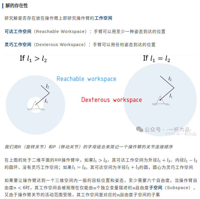
工作空间分析
研究笛卡尔空间中点的位置在操作臂的关节空间中是否有相应的解的问题,即分析操作臂的工作空间。回顾一下【机器人学导论】Ep4.操作臂逆运动学的内容:
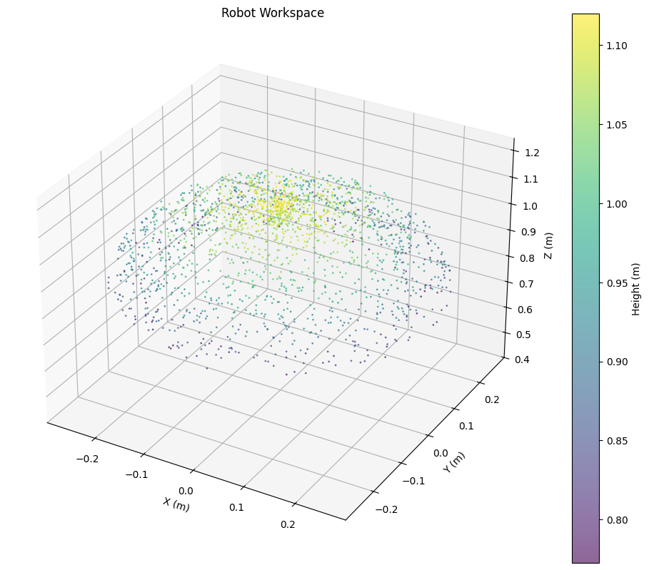
工作空间可以由直接计算求解,而在仿真软件下,为了进行可视化,我们可以通过蒙特卡洛方法在关节空间中随机采样,由MuJoCo模拟出采样点在笛卡尔空间中的位置,得到工作空间点云图:
def visualize_workspace(model: mujoco.MjModel, params: ArmParameters, samples: int = 1000):
    """
    可视化机械臂工作空间 / Visualize robot workspace
    """
    data = mujoco.MjData(model)
    workspace_points = []

    # 随机采样关节角度 / Random sample joint angles
    for _ in range(samples):
        # 在关节限位内随机采样 / Random sample within joint limits
        q = np.zeros(3)
        for i in range(3):
            q[i] = np.random.uniform(
                np.radians(params.joint_limits[i][0]),
                np.radians(params.joint_limits[i][1])
            )

        # 设置关节角度 / Set joint angles
        data.qpos[:3] = q
        mujoco.mj_forward(model, data)

        # 获取末端位置 / Get end effector position
        ee_pos = data.site('ee_site').xpos.copy()
        workspace_points.append(ee_pos)

    workspace_points = np.array(workspace_points)

    # 3D可视化 / 3D visualization
    fig = plt.figure(figsize=(12, 10))
    ax = fig.add_subplot(111, projection='3d')

    # 绘制工作空间点云 / Plot workspace point cloud
    scatter = ax.scatter(workspace_points[:, 0],
                        workspace_points[:, 1],
                        workspace_points[:, 2],
                        c=workspace_points[:, 2],  # 按高度着色 / Color by height
                        cmap='viridis',
                        alpha=0.6,
                        s=1)

    ax.set_xlabel('X (m)')
    ax.set_ylabel('Y (m)')
    ax.set_zlabel('Z (m)')
    ax.set_title("Robot Workspace")

    # 添加颜色条 / Add colorbar
    plt.colorbar(scatter, ax=ax, label='Height (m)')

    # 设置相等的轴比例 / Set equal axis scales
    max_range = np.array([workspace_points[:, 0].max() - workspace_points[:, 0].min(),
                         workspace_points[:, 1].max() - workspace_points[:, 1].min(),
                         workspace_points[:, 2].max() - workspace_points[:, 2].min()]).max() / 2.0

    mid_x = (workspace_points[:, 0].max() + workspace_points[:, 0].min()) * 0.5
    mid_y = (workspace_points[:, 1].max() + workspace_points[:, 1].min()) * 0.5
    mid_z = (workspace_points[:, 2].max() + workspace_points[:, 2].min()) * 0.5

    ax.set_xlim(mid_x - max_range, mid_x + max_range)
    ax.set_ylim(mid_y - max_range, mid_y + max_range)
    ax.set_zlim(0.4, mid_z + max_range)

    plt.show()

    return workspace_points

# 可视化工作空间 / Visualize workspace
workspace = visualize_workspace(arm_model, params, samples=2000)
机械臂控制与逆运动学分析
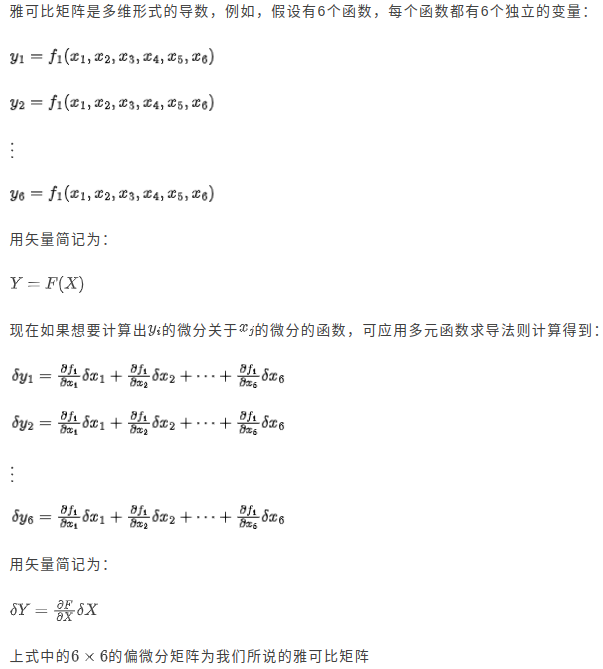
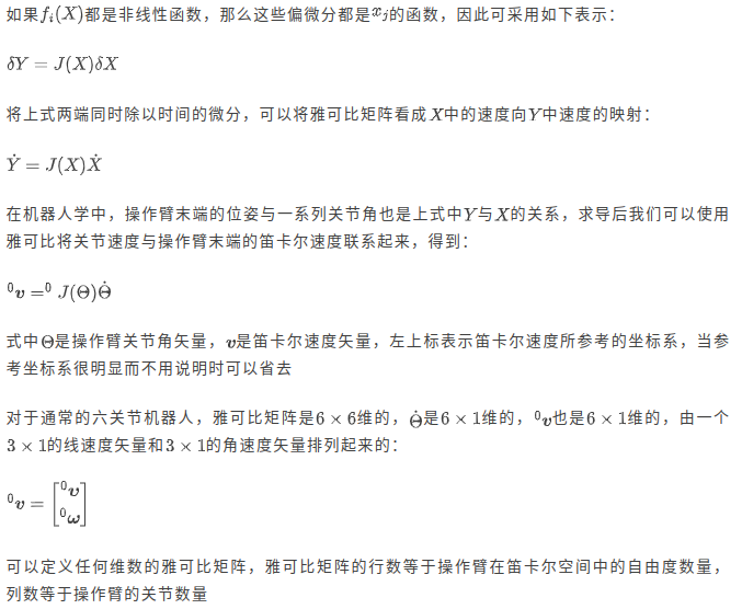
机械臂控制需要根据给定的目标末端位姿求解一系列关节角,即逆运动学分析。在【机器人学导论】Ep4.操作臂逆运动学中,我们给出了代数和几何两种解析法,这里我们再介绍一种利用雅克比矩阵迭代的数值法。回顾一下【机器人学导论】Ep5.雅克比:速度与静力中雅克比矩阵的概念:
MuJoCo提供了可以计算雅克比矩阵的mj_jacBody函数:
def compute_jacobian(model: mujoco.MjModel, data: mujoco.MjData) -> np.ndarray:
    """
    计算雅可比矩阵 / Compute Jacobian matrix
    """
    # 获取末端执行器的body id
    # Fix: Use mj_name2id instead of model.body()
    ee_body_id = mujoco.mj_name2id(model, mujoco.mjtObj.mjOBJ_BODY, 'end_effector')

    # 创建雅可比矩阵 / Create Jacobian matrices
    jacp = np.zeros((3, model.nv))  # 位置雅可比 / Position Jacobian
    jacr = np.zeros((3, model.nv))  # 旋转雅可比 / Rotation Jacobian

    # 计算雅可比 / Compute Jacobian
    mujoco.mj_jacBody(model, data, jacp, jacr, ee_body_id)

    return jacp
其中位置雅克比jacp是
3
×
1
3\times1
3×1线速度矢量
0
υ
^0\mathbf\upsilon
0υ,旋转雅克比jacr是
3
×
1
3\times1
3×1角速度矢量
0
ω
^0\mathbf\omega
0ω,各自代表在所有关节以单位速度运动的情况下指定id的刚体产生的相对于世界坐标系的线速度和自身旋转的角速度。这里我们不考虑姿态,因此只返回位置雅克比。
雅克比矩阵迭代法的原理是,末端执行器的位置变化量和关节的位置变化量之间存在如下微分关系
δ 0 P = 0 J ( Θ ) δ Θ \delta^0P=^0J(\Theta)\delta\Theta δ0P=0J(Θ)δΘ
在逆问题中,该关系则转换为
δ Θ ≈ 0 J + ( Θ ) δ 0 P \delta\Theta\approx^0J^+(\Theta)\delta^0P δΘ≈0J+(Θ)δ0P
其中
0
J
+
(
Θ
)
^0J^+(\Theta)
0J+(Θ)是
0
J
(
Θ
)
^0J(\Theta)
0J(Θ)的Moore-Penrose伪逆,对于无法计算逆矩阵的矩阵可以提供最佳近似解,可通过函数np.linalg.pinv()计算。
由于该计算只是小邻域下的局部线性近似,因此不宜将得到的 δ Θ \delta\Theta δΘ直接应用于关节变量,而是先乘上一个步长因子。更新完一次关节变量后,重新计算当前末端位置与目标位置之间的变化量以进行下一次更新,直至末端位置近似收敛于目标位置。
机械臂执行器采用比例积分微分控制(PID),即对于当前时刻的误差,控制量计算公式为
u ( t ) = K P e ( t ) + K I ∫ e ( t ) d t + K D d e ( t ) d t u(t)=K_Pe(t)+K_I\int e(t)\mathrm dt+K_D\frac{\mathrm de(t)}{\mathrm dt} u(t)=KPe(t)+KI∫e(t)dt+KDdtde(t)
其中 K P K_P KP, K I K_I KI和 K D K_D KD分别为比例增益、积分增益和微分增益。
详细的PID控制原理讲解请等待【控制原理】系列后续更新。
class RobotArmController:
    """
    机械臂控制器类 / Robot arm controller class
    """
    def __init__(self, model: mujoco.MjModel, data: mujoco.MjData):
        self.model = model
        self.data = data
        self.target_pos = np.array([0.2, 0.1, 0.8])  # 默认目标位置 / Default target position

        # PID参数 / PID parameters
        self.kp = np.array([2.0, 2.0, 2.0])  # 比例增益 / Proportional gain
        self.ki = np.array([0.1, 0.1, 0.1])  # 积分增益 / Integral gain
        self.kd = np.array([0.5, 0.5, 0.5])  # 微分增益 / Derivative gain

        self.error_integral = np.zeros(3)
        self.last_error = np.zeros(3)

    def inverse_kinematics_jacobian(self, target_pos: np.ndarray, max_iter: int = 100, tol: float = 1e-3):
        """
        使用雅可比方法的逆运动学 / Inverse kinematics using Jacobian method
        """
        for i in range(max_iter):
            # 当前末端位置 / Current end effector position
            ee_pos = self.data.site('ee_site').xpos

            # 位置误差 / Position error
            error = target_pos - ee_pos

            # 检查是否收敛 / Check convergence
            if np.linalg.norm(error) < tol:
                return self.data.qpos[:3].copy()

            # 计算雅可比 / Compute Jacobian
            J = compute_jacobian(self.model, self.data)

            # 计算伪逆 / Compute pseudo-inverse
            J_pinv = np.linalg.pinv(J)

            # 计算关节速度 / Compute joint velocities
            dq = J_pinv @ error

            # 更新关节角度 / Update joint angles
            self.data.qpos[:3] += 0.1 * dq  # 步长因子 / Step size factor

            # 应用关节限位 / Apply joint limits
            for j in range(3):
                self.data.qpos[j] = np.clip(
                    self.data.qpos[j],
                    self.model.jnt_range[j, 0],
                    self.model.jnt_range[j, 1]
                )

            # 更新仿真 / Update simulation
            mujoco.mj_forward(self.model, self.data)

        print(f"警告:逆运动学未收敛 / Warning: IK did not converge")
        return self.data.qpos[:3].copy()

    def pid_control(self, target_angles: np.ndarray, dt: float = 0.001):
        """
        PID控制器 / PID controller
        """
        # 当前关节角度 / Current joint angles
        current_angles = self.data.qpos[:3]

        # 计算误差 / Compute error
        error = target_angles - current_angles

        # PID计算 / PID calculation
        self.error_integral += error * dt
        error_derivative = (error - self.last_error) / dt

        # 控制输出 / Control output
        control = (self.kp * error +
                  self.ki * self.error_integral +
                  self.kd * error_derivative)

        # 更新历史误差 / Update error history
        self.last_error = error.copy()

        # 应用控制 / Apply control
        self.data.ctrl[:3] = control

        return control

# 创建控制器 / Create controller
controller = RobotArmController(arm_model, arm_data)

# 测试逆运动学 / Test inverse kinematics
target = np.array([0.2, 0.1, 0.8])
mujoco.mj_resetData(arm_model, arm_data)  # 重置状态 / Reset state
ik_solution = controller.inverse_kinematics_jacobian(target)

print(f"目标位置 / Target position: {target}")
print(f"IK解 / IK solution (degrees): {np.degrees(ik_solution)}")
print(f"实际末端位置 / Actual end position: {arm_data.site('ee_site').xpos}")
print(f"位置误差 / Position error: {np.linalg.norm(target - arm_data.site('ee_site').xpos):.4f}m")
目标位置 / Target position: [0.2 0.1 0.8]
IK解 / IK solution (degrees): [ 26.55555307  84.48810787 126.0462028 ]
实际末端位置 / Actual end position: [0.19986859 0.09989288 0.80094683]
位置误差 / Position error: 0.0010m
轨迹规划
回顾【机器人学导论】Ep7.轨迹生成
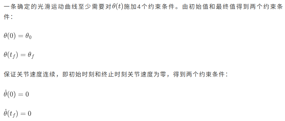
在这里,我们使用五次多项式进行轨迹规划,以限制 θ ¨ ( 0 ) = θ ¨ ( t f ) = 0 \ddot\theta(0)=\ddot\theta(t_f)=0 θ¨(0)=θ¨(tf)=0
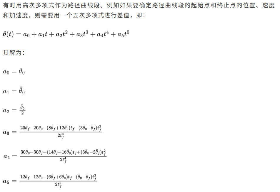
代入限制条件后化简结果如下
a 0 = a 1 = a 2 = 0 a_0=a_1=a_2=0 a0=a1=a2=0
a 3 = 10 θ f − θ 0 2 t f 3 \displaystyle a_3=10\frac{\theta_f-\theta_0}{2t_f^3} a3=102tf3θf−θ0
a 4 = − 15 θ f − θ 0 t f 4 \displaystyle a_4=-15\frac{\theta_f-\theta_0}{t_f^4} a4=−15tf4θf−θ0
a 5 = 6 θ f − θ 0 t f 5 \displaystyle a_5=6\frac{\theta_f-\theta_0}{t_f^5} a5=6tf5θf−θ0
def plan_joint_trajectory(start_angles: np.ndarray,
end_angles: np.ndarray,
duration: float,
dt: float = 0.001) -> Tuple[np.ndarray, np.ndarray]:
"""
五次多项式轨迹规划 / 5th order polynomial trajectory planning
"""
t = np.arange(0, duration, dt)
n_steps = len(t)
n_joints = len(start_angles)
# 初始化轨迹数组 / Initialize trajectory arrays
q_traj = np.zeros((n_steps, n_joints))
qd_traj = np.zeros((n_steps, n_joints))
for i in range(n_joints):
# 边界条件 / Boundary conditions
q0 = start_angles[i]
qf = end_angles[i]
# 五次多项式系数 / 5th order polynomial coefficients
# q(t) = a0 + a1*t + a2*t^2 + a3*t^3 + a4*t^4 + a5*t^5
# 初始和终止速度、加速度为0 / Initial and final velocity, acceleration = 0
T = duration
a0 = q0
a1 = 0
a2 = 0
a3 = 10 * (qf - q0) / (T**3)
a4 = -15 * (qf - q0) / (T**4)
a5 = 6 * (qf - q0) / (T**5)
# 计算轨迹 / Compute trajectory
for j, t_val in enumerate(t):
q_traj[j, i] = a0 + a1*t_val + a2*t_val**2 + a3*t_val**3 + a4*t_val**4 + a5*t_val**5
qd_traj[j, i] = a1 + 2*a2*t_val + 3*a3*t_val**2 + 4*a4*t_val**3 + 5*a5*t_val**4
return q_traj, qd_traj
def execute_trajectory(model: mujoco.MjModel,
data: mujoco.MjData,
controller: RobotArmController,
trajectory: np.ndarray,
record: bool = True) -> List[np.ndarray]:
"""
执行轨迹 / Execute trajectory
"""
frames = []
try:
renderer = mujoco.Renderer(model, width=640, height=480)
except Exception as e:
print(f"Renderer initialization failed: {e}")
renderer = mujoco.Renderer(model)
for i, target_angles in enumerate(trajectory):
# PID控制 / PID control
controller.pid_control(target_angles)
# 仿真步进 / Simulation step
mujoco.mj_step(model, data)
# 记录帧 / Record frame
if record and i % 10 == 0: # 每10步记录一帧 / Record every 10 steps
renderer.update_scene(data)
frames.append(renderer.render())
return frames
# 规划一个简单的轨迹 / Plan a simple trajectory
start_pos = np.array([0, 0, 0])
end_pos = np.array([np.pi/3, np.pi/4, -np.pi/6])
# 生成轨迹 / Generate trajectory
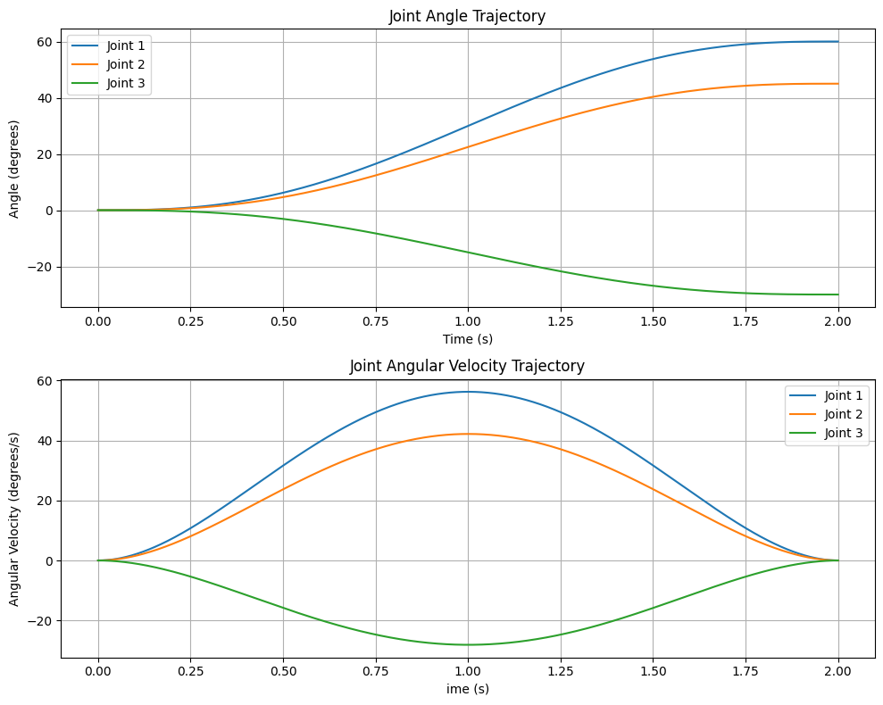
trajectory, velocity = plan_joint_trajectory(start_pos, end_pos, duration=2.0)
# 可视化轨迹 / Visualize trajectory
fig, (ax1, ax2) = plt.subplots(2, 1, figsize=(10, 8))
# 位置轨迹 / Position trajectory
time_points = np.linspace(0, 2, len(trajectory))
for i in range(3):
ax1.plot(time_points, np.degrees(trajectory[:, i]), label=f'Joint {i+1}')
ax1.set_xlabel('Time (s)')
ax1.set_ylabel('Angle (degrees)')
ax1.set_title("Joint Angle Trajectory")
ax1.legend()
ax1.grid(True)
# 速度轨迹 / Velocity trajectory
for i in range(3):
ax2.plot(time_points, np.degrees(velocity[:, i]), label=f'Joint {i+1}')
ax2.set_xlabel('Time (s)')
ax2.set_ylabel('Angular Velocity (degrees/s)')
ax2.set_title("Joint Angular Velocity Trajectory")
ax2.legend()
ax2.grid(True)
plt.tight_layout()
plt.show()
# 执行并录制 / Execute and record
print("执行演示动作... / Executing demo motion...")
frames = execute_trajectory(arm_model, arm_data, controller, trajectory, record=True)

# 显示动画 / Display animation
if frames:
    print(f"录制了 {len(frames)} 帧 / Recorded {len(frames)} frames")
    media.show_video(frames, fps=30)
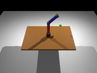
轨迹规划
仿真结果中,机械臂在目标位置附近产生较为持久的振荡,因此还需进行控制方面的优化,本系列暂不涉及。


 683
683

 被折叠的 条评论
为什么被折叠?
被折叠的 条评论
为什么被折叠?
 到【灌水乐园】发言


