


✅作者简介:热爱科研的Matlab仿真开发者,擅长数据处理、建模仿真、程序设计、完整代码获取、论文复现及科研仿真。
🍎 往期回顾关注个人主页:Matlab科研工作室
🍊个人信条:格物致知,完整Matlab代码及仿真咨询内容私信。
🔥 内容介绍
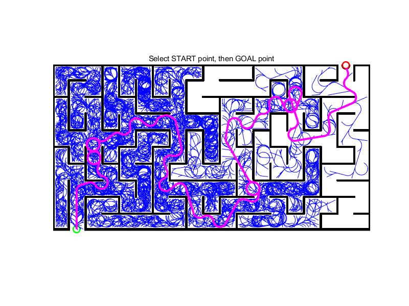
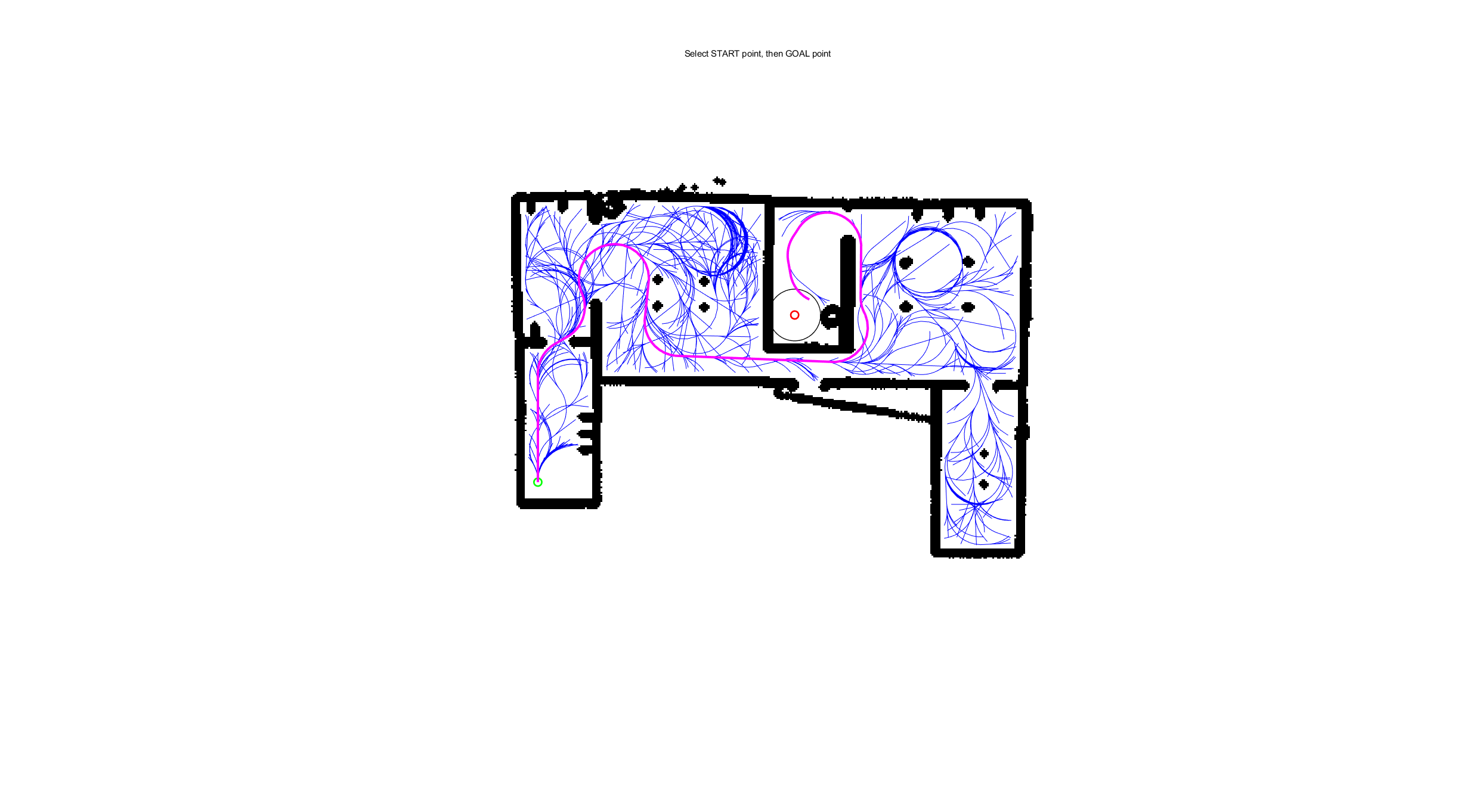
在机器人自主导航领域(如仓储 AGV、室外巡检机器人、工业机械臂),路径规划是核心功能之一,其目标是在含障碍物的地图环境中,找到一条从起点到终点的 “安全、最优、高效” 路径。不同场景对路径规划的需求差异显著 —— 仓储环境需 “最短路径 + 无碰撞”,室外越野场景需 “鲁棒性 + 快速响应”,工业场景需 “平滑路径 + 运动约束适配”。本文系统梳理 7 类主流路径规划算法:传统启发式算法(A*)、RRT 系列算法(Informer-RRT、RRT Connect、RRT SMART、Kinodynamic-RRT)及概率路标算法(PRM),构建统一地图建模框架,对比各算法在不同地图环境下的性能,为工程选型提供依据。
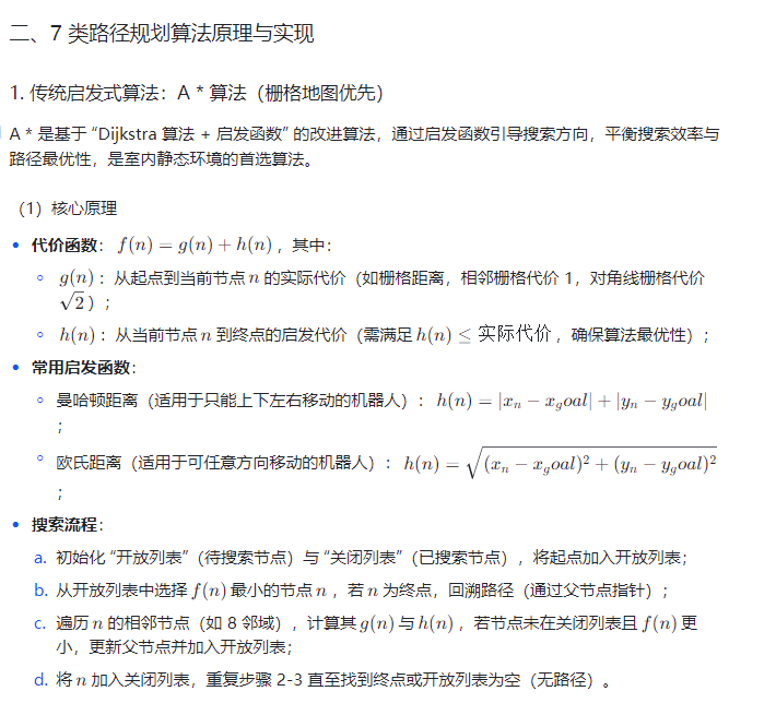
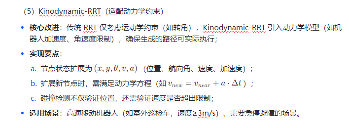
一、路径规划问题建模与地图环境定义
无论采用何种算法,路径规划的核心是将物理环境抽象为数学模型,明确 “状态空间 - 约束条件 - 优化目标” 三要素,为后续算法实现奠定基础。
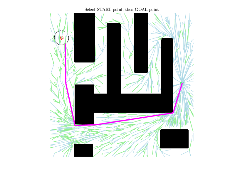
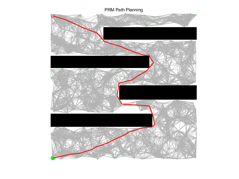
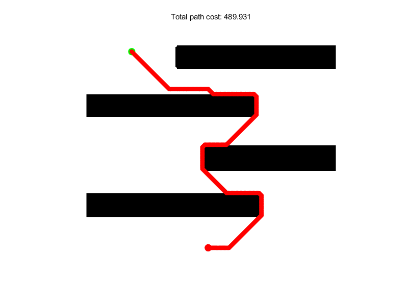
⛳️ 运行结果

📣 部分代码
clear;close all;
% Algorithm Parameters
max_iter = 20000;
step_size = 5;
radius = 25;
goal_radius = 6;
goal_bias=20;
% Options
show_runtime=1; % choose 1 to show the runtime plot (slow)
profile off;
% img1 = imread("Pictures/map_1_d.png");
% img1 = imread("Pictures/map_2_d.png");
% img1 = imread("Pictures/map_3_d.png");
img1 = imread("Pictures/map_4_d.png");
% img1 = imread("Pictures/maze3.jpg");
img = imbinarize(im2gray(img1), 0.8);
se = strel('disk', 1);
img = ~imdilate(~img, se);
map_size = size(img);
figure;
set(gcf, 'Position', [100, 100, 800, 600]);
imshow(img, 'InitialMagnification', 'fit');
hold on;
title('Select START point, then GOAL point');
% select by the user
[start_x, start_y] = ginput(1);
start = [round(start_x), round(start_y)];
plot(start(1), start(2), 'go', 'MarkerSize', 10, 'MarkerFaceColor', 'g');
pause(0.1);
[goal_x, goal_y] = ginput(1);
goal = [round(goal_x), round(goal_y)];
plot(goal(1), goal(2), 'ro', 'MarkerSize', 10, 'MarkerFaceColor', 'r');
pause(0.1);
% map1
% start= [8,116];
% goal = [274,115];
% % map2
% start= [9,79];
% goal = [262,281];
%
% % map3
% start= [6,6];
% goal = [5,298];
%
% % map4
% start= [11,74];
% goal = [191,181];
%
% % map,png
% start= [65,245];
% goal = [214,148];
plotCircle(goal, goal_radius)
%%%%%%%%%%%%%%%%%%% Main algorithm %%%%%%%%%%%%%
tic;
path = rrt_star_maze_path(img, start, goal, max_iter, step_size, radius, goal_radius,[show_runtime,goal_bias]);
elapsedtime = toc;
if ~isempty(path)
fprintf('Path found successfully! in %0.2f seconds\n', elapsedtime);
else
disp('No path found.');
end
%%
function path = rrt_star_maze_path(img, start, goal, max_iter, step_size, radius, goal_radius, varnargin)
if nargin > 7
show_runtime_plot = varnargin(1);
goal_bias = varnargin(2);
end
% Initialize variables
initial_path_found = false;
tree.nodes = start;
tree.parent = 0;
tree.cost = 0;
d = [];
best_goal_path = [];
best_goal_cost = inf; % Initialize best cost as infinity
% Calculate RRT* parameters
free_space = sum(sum(img)) / numel(img);
total_volume = size(img,1) * size(img,2);
gamma = 2 * sqrt(free_space * total_volume / pi);
for iter = 1:max_iter
if mod(iter,400)==0
disp('Current iteration is:')
disp(iter);
end
% Sample random point with goal bias
rand_point = random_sampling(img, goal, iter, goal_bias);
% Find nearest node
[nearest_idx, nearest_node] = find_nearest_node(tree.nodes, rand_point);
% Extend towards random point
new_node = extend_node(nearest_node, rand_point, step_size);
% Calculate current optimal radius
current_radius = get_optimal_radius(length(tree.nodes), gamma);
current_radius = max(current_radius,18);
% Check if path to new node is valid
if is_path_valid(img, nearest_node, new_node, step_size)
% Find nearby nodes for potential connections
[near_indices, near_nodes] = find_near_nodes(tree.nodes, new_node, current_radius);
% Choose parent node with minimum cost path
min_cost_idx = nearest_idx;
min_cost = tree.cost(nearest_idx) + node_distance(nearest_node, new_node);
% Check all nearby nodes for better parent
for i = 1:length(near_indices)
near_idx = near_indices(i);
near_node = near_nodes(i, :);
if is_path_valid(img, near_node, new_node, step_size)
potential_cost = tree.cost(near_idx) + node_distance(near_node, new_node);
if potential_cost < min_cost
min_cost_idx = near_idx;
min_cost = potential_cost;
end
end
end
% Add new node to tree
tree.nodes(end+1, :) = new_node;
tree.parent(end+1) = min_cost_idx;
tree.cost(end+1) = min_cost;
% Visualize new connection
if show_runtime_plot
plot([tree.nodes(min_cost_idx,1), new_node(1)], ...
[tree.nodes(min_cost_idx,2), new_node(2)], 'Color', [0.678, 0.847, 0.902], 'LineWidth', 1);
end
% Rewiring step
for i = 1:length(near_indices)
near_idx = near_indices(i);
near_node = near_nodes(i, :);
old_parent_idx = tree.parent(near_idx);
potential_new_cost = tree.cost(end) + node_distance(new_node, near_node);
if potential_new_cost < tree.cost(near_idx) && is_path_valid(img, new_node, near_node, step_size)
tree.parent(near_idx) = length(tree.nodes);
tree.cost(near_idx) = potential_new_cost;
if show_runtime_plot
% Erase old connection
plot([tree.nodes(old_parent_idx,1), near_node(1)], ...
[tree.nodes(old_parent_idx,2), near_node(2)], 'color', 'w', 'LineWidth', 1.5);
plot([new_node(1), near_node(1)], ...
[new_node(2), near_node(2)], 'Color', [0.565, 0.933, 0.565], 'LineWidth', 1.5);
drawnow limitrate;
end
end
end
% Check if goal is reached
if node_distance(new_node, goal) <= goal_radius
if ~initial_path_found
initial_path_found = true;
end
% Calculate the cost to reach goal through this new node
potential_goal_cost = tree.cost(end) + node_distance(new_node, goal);
if potential_goal_cost < best_goal_cost && is_path_valid(img, new_node, goal, step_size)
% Add goal to tree
tree.nodes(end+1, :) = goal;
tree.parent(end+1) = length(tree.nodes) - 1; % Parent is the new_node
tree.cost(end+1) = potential_goal_cost;
% Update best path and cost
[current_path, current_cost] = reconstruct_path(tree, length(tree.nodes));
best_goal_path = current_path;
best_goal_cost = current_cost;
% Update visualization
if show_runtime_plot
if ~isempty(d)
delete(d);
end
d = plot(best_goal_path(:,1), best_goal_path(:,2), 'r-', 'LineWidth', 3);
end
pause(1);
fprintf('New best path found with cost: %f\n', best_goal_cost);
end
% Remove goal node from tree to allow for future improvements
if tree.nodes(end, :) == goal
tree.nodes(end, :) = [];
tree.parent(end) = [];
tree.cost(end) = [];
end
end
end
end
% Return the best path found
if ~isempty(best_goal_path)
path = best_goal_path;
plot(path(:,1), path(:,2), 'r-', 'LineWidth', 3);
drawnow;
disp(['Path found with cost: ', num2str(best_goal_cost)]);
title(['Path found with cost: ', num2str(best_goal_cost)]); else
path = [];
disp('Path not found within max iterations');
end
end
%%%%%%%%%%%%%%%%%%%%%%%%%%% Algorithm Helpers %%%%%%%%%%%%%%%%%%%%%%%%%%%%
% Find the nearest node in the tree to a given point
function [nearest_idx, nearest_node] = find_nearest_node(nodes, point)
distances = sqrt(sum((nodes - point).^2, 2));
[~, nearest_idx] = min(distances);
nearest_node = nodes(nearest_idx, :);
end
% Find nodes within a specified radius of the new node
function [near_indices, near_nodes] = find_near_nodes(nodes, new_node, radius)
distances = sqrt(sum((nodes - new_node).^2, 2));
near_indices = find(distances <= radius);
near_nodes = nodes(near_indices, :);
end
%steer
function new_node = extend_node(nearest_node, rand_point, step_size)
direction = (rand_point - nearest_node) / node_distance(rand_point , nearest_node);
new_node = nearest_node + direction * step_size;
new_node = round(new_node);
end
function dist = node_distance(node1, node2)
% Ensure both nodes are in the same coordinate system
if size(node1, 1) > 2 % If using matrix coordinates
node1 = node1(:, [2 1]); % Swap x,y to match A* coordinate system
node2 = node2(:, [2 1]);
end
dist = sqrt(sum((node1 - node2).^2, 2));
end
%%%%%%%%%%%%%%%%%%%%%%%%%%%%%% colision check %%%%%%%%%%%%%%
function is_free = is_path_valid1(img,x1, x2 ,step_size)
num_points = round(step_size/0.5);
x_points = round(linspace(round(x1(1)), round(x2(1)), num_points));
y_points = round(linspace(round(x1(2)), round(x2(2)), num_points));
x_points = max(1, min(size(img, 2), x_points)); % Clamp to [1, width]
y_points = max(1, min(size(img, 1), y_points)); % Clamp to [1, height]
is_free = all(arrayfun(@(x, y) img(y, x), x_points, y_points)); % 1=free, 0=obstacle
end
% Faster
function is_free = is_path_valid(img, x1, x2, step_size)
% Calculate number of points
num_points = round(step_size/0.05);
% Create vectors directly using multiplication and addition
% This avoids linspace overhead
t = (0:num_points-1)' / (num_points-1);
x_points = round(x1(1) + (x2(1) - x1(1)) * t);
y_points = round(x1(2) + (x2(2) - x1(2)) * t);
% Clamp values using min/max
x_points = max(1, min(size(img, 2), x_points));
y_points = max(1, min(size(img, 1), y_points));
% Convert to linear indices for faster access
linear_indices = sub2ind(size(img), y_points, x_points);
% Check all points at once using linear indexing
is_free = all(img(linear_indices));
end
%%%%%%%%%%%%%%%%%%%% Reconstruct the path to goal %%%%%%%%%%%%%%%%%%%%%%%%%
function [path, actual_cost] = reconstruct_path(tree, goal_idx)
path = tree.nodes(goal_idx, :);
current_idx = goal_idx;
actual_cost = 0;
while tree.parent(current_idx) ~= 0
parent_idx = tree.parent(current_idx);
% Add the actual segment cost
actual_cost = actual_cost + node_distance(tree.nodes(current_idx, :), tree.nodes(parent_idx, :));
% Add parent node to path
current_idx = parent_idx;
path = [tree.nodes(current_idx, :); path];
end
end
function path = reconstruct_path2(tree, goal_idx)
path = tree.nodes(goal_idx, :);
current_idx = goal_idx;
while tree.parent(current_idx) ~= 0
current_idx = tree.parent(current_idx);
path = [tree.nodes(current_idx, :); path];
end
end
%%%%%%%%%%%%%%%%%%%%%%%%%%%% random sampling strategies %%%%%%%%%%%%%%%%%%
function rand_point = improved_random_sampling(img, start, goal, iter, max_iter)
goal_bias_prob = 0.1; % Probability of sampling the goal directly
gaussian_sampling_prob = 0.2; % Probability of Gaussian sampling
% Random number to decide sampling strategy
sample_strategy = rand();
% Goal biasing: directly sample goal with a small probability
if sample_strategy < goal_bias_prob
rand_point = goal;
return;
end
% Gaussian-like sampling around promising regions
if sample_strategy < (goal_bias_prob + gaussian_sampling_prob)
% Calculate progress towards goal (normalized)
progress = iter / max_iter;
% Adaptive sampling range
range_x = max(size(img, 2) * (1 - progress), 50);
range_y = max(size(img, 1) * (1 - progress), 50);
% Center between start and goal
center_x = (start(1) + goal(1)) / 2;
center_y = (start(2) + goal(2)) / 2;
% Use uniform distribution with reduced range as pseudo-Gaussian
rand_point = [
max(1, min(size(img, 2), round(center_x + (rand()-0.5) * range_x))), ...
max(1, min(size(img, 1), round(center_y + (rand()-0.5) * range_y)))
];
return;
end
% Uniform random sampling for the rest
rand_point = [
randi([1, size(img,2)]), ...
randi([1, size(img,1)])
];
end
function rand_point = random_sampling(img, goal, iter, goal_bias)
if nargin < 3
goal_bias = 10;
end
if mod(iter,goal_bias) ==0 % Bias towards goal
rand_point = goal;
else
rand_point = [randi([1, size(img,2)]), randi([1, size(img,1)])];
end
end
%%%%%%%%%%%%%%%%%%%% Helper Functions %%%%%%%%%%%%%%%%%%%%%%%%%
function radius = get_optimal_radius(n, gamma)
if n < 2
radius = inf;
return;
end
d = 2;
radius = gamma * (log(n)/n)^(1/d);
end
function plotCircle(center, radius)
% Validate inputs
if length(center) ~= 2 || ~isnumeric(center)
error('Center must be a numeric vector of size 1x2.');
end
if ~isscalar(radius) || ~isnumeric(radius) || radius <= 0
error('Radius must be a positive numeric scalar.');
end
% Generate points for the circle
theta = linspace(0, 2*pi, 100); % 100 points around the circle
x = center(1) + radius * cos(theta);
y = center(2) + radius * sin(theta);
plot(x, y, 'k-', 'LineWidth', 1); % Circle in blue with a line width of 2
end
🔗 参考文献
🎈 部分理论引用网络文献,若有侵权联系博主删除
👇 关注我领取海量matlab电子书和数学建模资料
🏆团队擅长辅导定制多种科研领域MATLAB仿真,助力科研梦:
🌟 各类智能优化算法改进及应用
生产调度、经济调度、装配线调度、充电优化、车间调度、发车优化、水库调度、三维装箱、物流选址、货位优化、公交排班优化、充电桩布局优化、车间布局优化、集装箱船配载优化、水泵组合优化、解医疗资源分配优化、设施布局优化、可视域基站和无人机选址优化、背包问题、 风电场布局、时隙分配优化、 最佳分布式发电单元分配、多阶段管道维修、 工厂-中心-需求点三级选址问题、 应急生活物质配送中心选址、 基站选址、 道路灯柱布置、 枢纽节点部署、 输电线路台风监测装置、 集装箱调度、 机组优化、 投资优化组合、云服务器组合优化、 天线线性阵列分布优化、CVRP问题、VRPPD问题、多中心VRP问题、多层网络的VRP问题、多中心多车型的VRP问题、 动态VRP问题、双层车辆路径规划(2E-VRP)、充电车辆路径规划(EVRP)、油电混合车辆路径规划、混合流水车间问题、 订单拆分调度问题、 公交车的调度排班优化问题、航班摆渡车辆调度问题、选址路径规划问题、港口调度、港口岸桥调度、停机位分配、机场航班调度、泄漏源定位、冷链、时间窗、多车场等、选址优化、港口岸桥调度优化、交通阻抗、重分配、停机位分配、机场航班调度、通信上传下载分配优化
🌟 机器学习和深度学习时序、回归、分类、聚类和降维
2.1 bp时序、回归预测和分类
2.2 ENS声神经网络时序、回归预测和分类
2.3 SVM/CNN-SVM/LSSVM/RVM支持向量机系列时序、回归预测和分类
2.4 CNN|TCN|GCN卷积神经网络系列时序、回归预测和分类
2.5 ELM/KELM/RELM/DELM极限学习机系列时序、回归预测和分类
2.6 GRU/Bi-GRU/CNN-GRU/CNN-BiGRU门控神经网络时序、回归预测和分类
2.7 ELMAN递归神经网络时序、回归\预测和分类
2.8 LSTM/BiLSTM/CNN-LSTM/CNN-BiLSTM/长短记忆神经网络系列时序、回归预测和分类
2.9 RBF径向基神经网络时序、回归预测和分类
2.10 DBN深度置信网络时序、回归预测和分类
2.11 FNN模糊神经网络时序、回归预测
2.12 RF随机森林时序、回归预测和分类
2.13 BLS宽度学习时序、回归预测和分类
2.14 PNN脉冲神经网络分类
2.15 模糊小波神经网络预测和分类
2.16 时序、回归预测和分类
2.17 时序、回归预测预测和分类
2.18 XGBOOST集成学习时序、回归预测预测和分类
2.19 Transform各类组合时序、回归预测预测和分类
方向涵盖风电预测、光伏预测、电池寿命预测、辐射源识别、交通流预测、负荷预测、股价预测、PM2.5浓度预测、电池健康状态预测、用电量预测、水体光学参数反演、NLOS信号识别、地铁停车精准预测、变压器故障诊断
🌟图像处理方面
图像识别、图像分割、图像检测、图像隐藏、图像配准、图像拼接、图像融合、图像增强、图像压缩感知
🌟 路径规划方面
旅行商问题(TSP)、车辆路径问题(VRP、MVRP、CVRP、VRPTW等)、无人机三维路径规划、无人机协同、无人机编队、机器人路径规划、栅格地图路径规划、多式联运运输问题、 充电车辆路径规划(EVRP)、 双层车辆路径规划(2E-VRP)、 油电混合车辆路径规划、 船舶航迹规划、 全路径规划规划、 仓储巡逻、公交车时间调度、水库调度优化、多式联运优化
🌟 无人机应用方面
无人机路径规划、无人机控制、无人机编队、无人机协同、无人机任务分配、无人机安全通信轨迹在线优化、车辆协同无人机路径规划、
🌟 通信方面
传感器部署优化、通信协议优化、路由优化、目标定位优化、Dv-Hop定位优化、Leach协议优化、WSN覆盖优化、组播优化、RSSI定位优化、水声通信、通信上传下载分配
🌟 信号处理方面
信号识别、信号加密、信号去噪、信号增强、雷达信号处理、信号水印嵌入提取、肌电信号、脑电信号、信号配时优化、心电信号、DOA估计、编码译码、变分模态分解、管道泄漏、滤波器、数字信号处理+传输+分析+去噪、数字信号调制、误码率、信号估计、DTMF、信号检测
🌟电力系统方面
微电网优化、无功优化、配电网重构、储能配置、有序充电、MPPT优化、家庭用电、电/冷/热负荷预测、电力设备故障诊断、电池管理系统(BMS)SOC/SOH估算(粒子滤波/卡尔曼滤波)、 多目标优化在电力系统调度中的应用、光伏MPPT控制算法改进(扰动观察法/电导增量法)、电动汽车充放电优化、微电网日前日内优化、储能优化、家庭用电优化、供应链优化
🌟 元胞自动机方面
交通流 人群疏散 病毒扩散 晶体生长 金属腐蚀
🌟 雷达方面
卡尔曼滤波跟踪、航迹关联、航迹融合、SOC估计、阵列优化、NLOS识别
🌟 车间调度
零等待流水车间调度问题NWFSP 、 置换流水车间调度问题PFSP、 混合流水车间调度问题HFSP 、零空闲流水车间调度问题NIFSP、分布式置换流水车间调度问题 DPFSP、阻塞流水车间调度问题BFSP
👇


 1188
1188

 被折叠的 条评论
为什么被折叠?
被折叠的 条评论
为什么被折叠?
 到【灌水乐园】发言


