基于Matlab模拟宇宙射线μ

✅作者简介：热爱科研的Matlab仿真开发者，修心和技术同步精进，matlab项目合作可私信。

🍎个人主页：Matlab科研工作室

🍊个人信条：格物致知。

更多Matlab仿真内容点击👇

智能优化算法       神经网络预测       雷达通信       无线传感器        电力系统

信号处理              图像处理               路径规划       元胞自动机        无人机 

⛄ 内容介绍

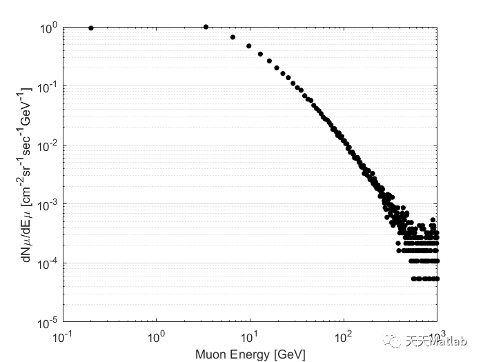
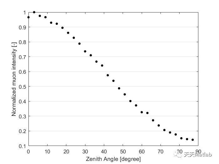
The cosmic ray muon (CRM) simulator provides stochastic results based on the two semi-empirical models: (1) muon energy distribution and (2) zenith angle distribution. Both energy and zenith angle distribution models are developed based on analytical studies and experimental data.

⛄ 部分代码

%___________________________________________________________

%

%                        MuSpect.m

%___________________________________________________________

%   "MuSpect.m" provides a cosmic ray muon (CRM) energy distribution with a

%  ragne from 0.2 GeV to the user-defiend maximum energy, MaxE (< 2,000 GeV).

%  The maximum muon energy is limited upto 2,000 [GeV] or 2 [TeV] because

%  the uncertainty level of CRM count rate is too high. Very high CRM

%  energy, > 2 TeV, is extremely rare event, especially at sea level.

%  Details for the model, please read:

%   [1] Cosmic Rays and Particle Physics, 2nd Ed., (2016), T. Gaisser, R. Engel, E. Resconi

%   [2] Review of Particle Physics, (2022), R.L. Workman et al (PDG), Prog. Theor. Exp. Phys. 

%

%  Inputs:

%  (1) MaxE: Maximum CRM energy to simulate [GeV]

%  (2) ZenAngle: Zenith angle (pointing angle of a detector surface) [deg]

%  (3) iffig: show (=1) or suppress (=0) figures.

%  For example,

%  >>    [dNdE, E_mu, sigma_E, ZenAngle] = MuSpect(1000,10,1)

%

%================================================================

if MaxE > 2000

    disp('Please adjust your input, Maximum Energy');

    return ;

end

sigma_E = 0.1;

E_mu = linspace(0.2 + sigma_E/2, MaxE-sigma_E/2, 1E5); %[GeV]

% Minimun and maximum degrees are slightly adjusted to take into account 

% +-0.05 GeV uncertainty during the random generation process.

ZenAng = ZenAngle * (pi/180);  % Degree -> radian

% Total atmospheric depth at sea level

X0 = 1030; % [g/cm2]

% Energy loss rate of muon through the atmosphere

alpha = 2E-3; % [GeV/g/cm2]

% Integral spectral index of the cosmic-ray spectrum

Gamma = 1.7;

% Spectrum-weighted moment for a "i" to produce "j" when Z_ji 

Z_NN = 0.3;

Z_Npi = 0.08;

Z_Nkp = 0.15 * Z_Npi;

% Mass ratio, muon to pion/kaon

r_pi = 0.573; % (m_mu/m_pi)^2

r_kp = 0.046; % (m_mu/m_kp)^2

% Characteristic length for exponential attenuation in the atmosphere.

% Char lengths depend on particle energy as shown in data set below.

Lambda_N_data  = [120 115 106 97];   % [g/cm2] When E = [1E2 1E3 1E4 1E5] GeV

Lambda_pi_data = [155 148 135 114];

Lambda_kp_data = [160 147 133 114];

% Critical energy

epsilon_pi = 115; % [GeV]

epsilon_kp = 850; 

epsilon_mu = 1;

% Energy dependent numerical values

% Boundary condition, the initial flux of CRM at the slant depth is X 

% in the atmosphere with energies in the interval E to E+dE

N0 = 1.7*E_mu.^(-2.7);

%

p1 = epsilon_mu./(E_mu.*cos(ZenAng)+alpha*X0);

% Lambdas depend on E_mu. Curve-fitting for the approximation.

Lambda_N = -13.31.*E_mu.^(0.1061)+142;

Lambda_pi = -3.714.*E_mu.^(0.2289)+165.8;

Lambda_kp = -36.28.*E_mu.^(0.08816)+214.2;

%

A_pimu = Z_Npi*(1-(r_pi).^(Gamma+1))./((1-r_pi).*(Gamma+1));

B_pimu = (1+(Gamma+1)^-1).*((1-(r_pi).^(Gamma+1))./(1-(r_pi).^(Gamma+2))).* ((Lambda_pi - Lambda_N)./(Lambda_pi.*log(Lambda_pi./Lambda_N)));

A_kpmu = Z_Nkp*(1-(r_kp).^(Gamma+1))./((1-r_kp).*(Gamma+1));

B_kpmu = (1+(Gamma+1)^-1).*((1-(r_kp).^(Gamma+1))./(1-(r_kp).^(Gamma+2))).* ((Lambda_kp - Lambda_N)./(Lambda_kp.*log(Lambda_kp./Lambda_N)));

% Suppression Factor

S = (Lambda_N.* cos(ZenAng)./X0).^p1 .* (E_mu./(E_mu+(alpha*X0./cos(ZenAng)))).^(p1+Gamma+1).* gamma(p1+1);

% Differential muon flux [cm-2 sr-1 sec-1 GeV-1]

dNdE = (S.*(N0./(1-Z_NN))).*((A_pimu./(1+B_pimu.*cos(ZenAng).*(E_mu./epsilon_pi)))...

        + (0.635.*A_kpmu./(1+B_kpmu.*cos(ZenAng).*(E_mu./epsilon_kp))));

    

    if iffig == 1

plot(E_mu,dNdE.*(E_mu.^3),'LineWidth', 2)

%                    ^^^

% Exponent can be adjusted for user's preference to display the figure.

hold on

set(gca, 'XScale', 'log')

set(gca, 'YScale', 'log')

ax = gca;

ax.YGrid = 'on';

ax.GridLineStyle = '-';

xlabel('Muon Energy [GeV]')

ylabel('E^3{\mu} dN{\mu}/dE{\mu} [cm^{-2}sr^{-1}sec^{-1}GeV^2]')    

    end

end

%===========================================================

%

%                       END

%

%===========================================================

⛄ 运行结果

⛄ 参考文献

[1] Cosmic Rays and Particle Physics, 2nd Ed., (2016), T. Gaisser, R. Engel, E. Resconi.

[2] Review of Particle Physics, (2022), R.L. Workman et al (PDG), Prog. Theor. Exp. Phys. 

[3] A New Semi-Empirical Model for Cosmic Ray Muon Flux Estimation, (2022) J.Bae, S. Chatzidakis, Prog. Theor. Exp. Phys.

⛄ 完整代码

❤️部分理论引用网络文献，若有侵权联系博主删除

❤️ 关注我领取海量matlab电子书和数学建模资料