图像异常检测评估指标-分割性能

图像异常检测性能评估-分割性能

In the present work, we study anomaly segmentation algorithms that are capable of returning a real-valued anomaly score for each pixel in a test image. Larger values shall indicate a higher likelihood of a pixel to be anomalous. Let us consider a test set T : = { I 1 , … , I n } T:=\{I_1,\ldots,I_n\} T:={I1​,…,In​} of $n$ images. We denote the anomaly scores for a test image $I_i$ at pixel $p$ as $A_i(p)\in \mathbb{R}.$ For each test image, there exists a pixel-precise ground truth G i ( p ) ∈ { 0 , 1 } G_i(p)\in\{0,1\} Gi​(p)∈{0,1} that indicates whether an anomaly is present i.e., $G_i(p)=1$, or not, i.e., $G_i(p)=0.$ In order to compare the anomaly scores with the ground truth data, it is necessary to pick a threshold $t\in \mathbb{R}$ to make a binary decision. A pixel is predicted to be anomalous if and only if $A_i(p)>t.$ Figure 1 shows an exemplary anomaly map generated by one of the evaluated methods for an anomalous input image of class metal nut. It further depicts the corresponding ground truth of the color defect as well as the binary segmentation results for decreasing thresholds as a contour plot.

1. 混淆矩阵

Evaluating the performance of anomaly segmentation algorithms on a per-pixel level treats the classification outcome of each pixel as equally important.

A pixel can be classified as either a true positive (TP), false positive (FP), true negative (TN), or false negative (FN). For each of the four cases the total number of pixels on the test dataset T is computed as:
TP = ∑ i = 1 n ∣ { p ∣ G i ( p ) = 1 } ∩ { p ∣ A i ( p ) > t } ∣ , ( 1 ) FP = ∑ i = 1 n ∣ { p ∣ G i ( p ) = 0 } ∩ { p ∣ A i ( p ) > t } ∣ , ( 2 ) T N = ∑ i = 1 n ∣ { p ∣ G i ( p ) = 0 } ∩ { p ∣ A i ( p ) ≤ t } ∣ , ( 3 ) FN = ∑ i = 1 n ∣ { p ∣ G i ( p ) = 1 } ∩ { p ∣ A i ( p ) ≤ t } ∣ . ( 4 ) \begin{gathered} \text{TP} =\sum_{i=1}^n\Big| \{p\mid G_i(p)=1\}\cap\{p\mid A_i(p)>t\}\Big|, \quad{(1)} \\ \text{FP} =\sum_{i=1}^n\big|\left\{p\mid G_i(p)=0\right\}\cap\{p\mid A_i(p)>t\}\big|, \quad{(2)} \\ TN =\sum_{i=1}^n\Big| \{p\mid G_i(p)=0\}\cap\{p\mid A_i(p)\leq t\}\Big|, \quad{(3)} \\ \text{FN} =\sum_{i=1}^n\Big| \{p\mid G_i(p)=1\}\cap\{p\mid A_i(p)\leq t\}\Big|. \quad{(4)} \end{gathered} TP=i=1∑n​ ​{p∣Gi​(p)=1}∩{p∣Ai​(p)>t} ​,(1)FP=i=1∑n​ ​{p∣Gi​(p)=0}∩{p∣Ai​(p)>t} ​,(2)TN=i=1∑n​ ​{p∣Gi​(p)=0}∩{p∣Ai​(p)≤t} ​,(3)FN=i=1∑n​ ​{p∣Gi​(p)=1}∩{p∣Ai​(p)≤t} ​.(4)​

2. 特定阈值下的评估指标

2.1 Pixel-Level Metrics

（1）TPR

$$\mathrm{TPR}=\frac{\mathrm{TP}}{\mathrm{TP}+\mathrm{FN}},(5)$$

（2）FPR

$$\mathrm{FPR}=\frac{\mathrm{FP}}{\mathrm{FP}+\mathrm{TN}},(6)$$

（3）PRC(Precision)

$$\mathrm{PRC}=\frac{\mathrm{TP}}{\mathrm{TP}+\mathrm{FP}},(7)$$

（4）IoU

In the context of anomaly segmentation, one considers the set of all anomalous predictions, i.e., P = ⋃ i = 1 n { p ∣ A i ( p ) > t } P=\bigcup_{i=1}^n\{p\mid A_i(p)>t\} P=⋃i=1n​{p∣Ai​(p)>t}, and the set of all ground truth pixels that are labeled as anomalous, i.e., G = ⋃ i = 1 n { p ∣ G i ( p ) = 1 } . G=\bigcup_i=1^n\{p\mid G_i(p)=1\}. G=⋃i​=1n{p∣Gi​(p)=1}. Analogously to the relative measures above, the IoU for the class ‘anomalous’ can also be expressed in terms of absolute pixel classification measures:

$$\mathrm{IoU}=\frac{|P\cap G|}{|P\cup G|}=\frac{\mathrm{TP}}{\mathrm{TP}+\mathrm{FP}+\mathrm{FN}},(8)$$

（5）总结

All these measures have the advantage that they are easy and efficient to compute. However, treating each pixel as entirely independent introduces a bias towards large anomalous regions. Detecting a single defect with a large area can make up for the failure to detect numerous smaller defects.

2.2 Region-Level Metrics

Instead of treating every pixel independently, region-level metrics average the performance over each connected component of the ground truth. This is especially useful if the detection of smaller anomalies is considered equally important as the detection of larger ones.

（1）PRO

First, for each test image the ground truth is decomposed into its connected components. Let $C_{i,k}$ denote the set of pixels marked as anomalous for a connected component $k$ in the ground truth image $i$ and $P_i$ denote the set of pixels predicted as anomalous for a threshold $t.$ The per-region overlap can then be computed as

$$\mathrm{PRO}=\frac{1}{N}\sum _i\sum _k\frac{|P_i\cap C_{i,k}|}{|C_{i,k}|},(9)$$

where $N$ is the number of total ground truth components in the evaluated dataset. The PRO metric is closely related to the TPR. The crucial difference is that the PRO metric averages the TPR over each ground truth region instead of averaging over all image pixels.

分析anomalib的pro.py，理出针对特定阈值计算PRO指标的计算流程如下：

（分析代码可知，PRO指标其实就是各连通区域的平均召回率，因此它是Region-Level Metrics）

3. 阈值无关的评估指标

All of the metrics listed above depend on the previous selection of a suitable threshold t, which is a challenging problem in practice . If the threshold determination fails, the performance metrics might give a skewed picture of the real performance of a method. Therefore, one often evaluates the above metrics at multiple distinct thresholds. Furthermore, it is desirable to compare two metrics simultaneously since, for example, a high TPR is only useful if the corresponding FPR is low. A way to achieve this is to plot two metrics against each other and compute the area under the resulting curve.

3.1 Per-Pixel Metrics

Per-Pixel Metrics 将会平等对待每个像素，导致：面积大的异常区域对评估结果的影响大于面积小的异常区域

（1）ROC Curve

the receiver operator characteristic (ROC), which plots the FPR versus the TPR.

（2）PR Curve

the precision–recall curve (PR), which plots the TPR(recall) versus the precision.

（3）IoU Curve

the IoU curve, which shows the FPR versus the IoU.

3.2 Per-Region Metrics

Per-Region Metrics 将会平等对待不同大小的区域，导致：面积大的异常区域和面积小的异常区域对评估结果的影响相等

（1）PRO Curve

the PRO curve, which plots the FPR versus the PRO

3.3 总结

It is important to note that the test split of our anomaly detection dataset is highly imbalanced in the sense that the number of anomalous pixels is significantly smaller than the number of anomaly-free ones.

Therefore, thresholds that yield a large FPR result in segmentation results that are no longer meaningful. This is especially the case for industrial applications. There, large false positive rates would lead to a large amount of defect-free parts being wrongly rejected.

The thresholds were selected such that they result in different false positive rates on the input image, ranging from 1%, for which the defect is well detected, to 100%, where the entire image is segmented as anomalous.

Therefore, we additionally include metrics in our evaluations that compute the area under the curves only up to a certain false positive rate. To ensure that the maximum attainable values of this performance measure is equal to 1, we normalize the resulting area.

Since the PR curve has been specifically designed to handle large class imbalances and does not use the FPR in its computation, we always evaluate its entire area.

4. 总结如何评估分割性能

4.1 评估顺序

1. 先利用阈值无关的指标（PRO Curve、ROC Curve、PR Curve、IoU Curve的形态以及曲线下面积）选择更有潜力的算法
2. 在1选出最有潜力算法的基础上，选择最优的阈值发挥出它最大的潜力（以适应实际应用场景）
3. 计算该特定阈值下的相关评估指标（TPR(Recall)、FPR(误诊率)、PRC(Precision)、IoU），对应应用场景进行分析

4.2 具体操作

1. 阈值无关的指标主要看哪些？（排名有先后，如果只能选择一个就选择PRO Curve）

   1. PRO Curve：平等对待不同大小的区域
   2. ROC Curve：平等对待每个像素（如果数据集中异常的面积差异不大，可以用这个）
   3. PR Curve：异常像素和正常像素数量不平衡用这个也合适
   4. IoU Curve

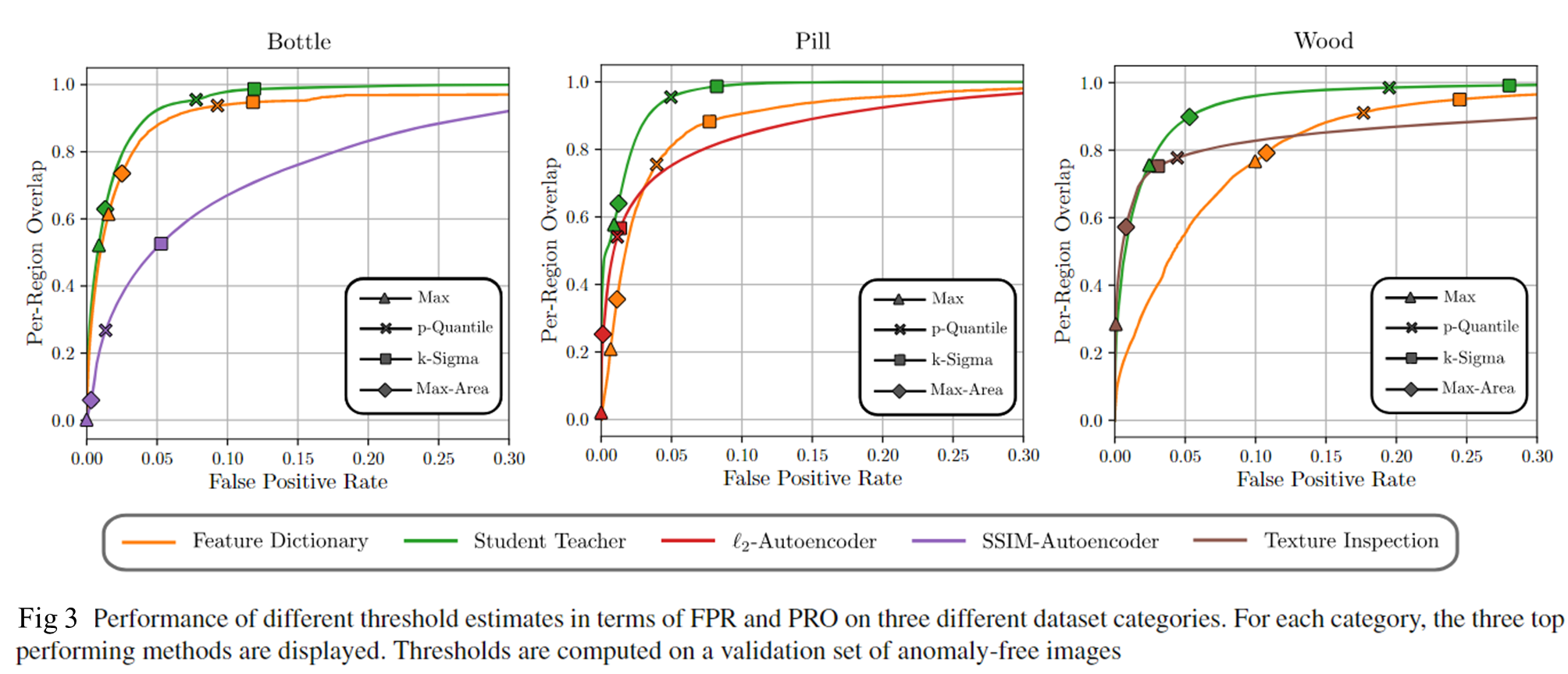
2. 如何选择最优阈值？（排名有先后）—— 选择阈值后，可以在PRO Curve上标出对应的点

   1. p-Quantile Threshold

   2. k-Sigma Threshold

   3. Maximum Threshold

   4. Max-Area Threshold

      

3. 计算该特定阈值下的相关评估指标（TPR(Recall)、FPR(误诊率)、PRC(Precision)、IoU），对应应用场景进行分析

5. 参考资料

1. WANG L, ZHANG D, GUO J, et al. Image Anomaly Detection Using Normal Data Only by Latent Space Resampling[J/OL]. Applied Sciences, 2020: 8660. http://dx.doi.org/10.3390/app10238660. DOI:10.3390/app10238660.
   n Using Normal Data Only by Latent Space Resampling[J/OL]. Applied Sciences, 2020: 8660. http://dx.doi.org/10.3390/app10238660. DOI:10.3390/app10238660.
2. The MVTec Anomaly Detection Dataset: A Comprehensive Real-World Dataset for Unsupervised Anomaly Detection