


 该博客基于PyTorch实现作业中的多类别分类问题。介绍了Logistic模型,输入数据为5000x400,有10个类别。阐述了读取数据的方法,采用Logistic回归,选择CrossEntropyLoss损失函数和Adam优化方法。还尝试修改Linear层初始化权重和weight_decay值以提升准确率。
目录
Exercise 3: Multi-class Classification
Exercise 3: Multi-class Classification
基于pytorch,只实现作业中多类别分类问题。
需要用到的库
import numpy as np
import scipy.io
import matplotlib.pyplot as plt
import torch
import torch.nn as nn
1. Logistic 模型
输入的数据为5000x400,共有10个类别,故线性层的大小为:nn.Linear(400, 10),最后使用softmax激活,所有的权重初始化为0。
input_layer_size  = 400  # 20x20 Input Images of Digits
num_labels = 10          # 10 labels, from 1 to 10


class Logistic(nn.Module):
    def __init__(self):
        super(Logistic, self).__init__()
        self.linear = nn.Linear(input_layer_size, num_labels)
        self.softmax = nn.Softmax(dim=1)
        nn.init.constant_(self.linear.weight, 0)
        nn.init.constant_(self.linear.bias, 0)

    def forward(self,x):
        out = self.linear(x)
        out = self.softmax(out)
        return out
2. 读取数据
读取数据方法与之前的函数相同详见博客:
https://blog.youkuaiyun.com/linghu8812/article/details/89786169
3.Logistic 回归
模型选择之前定义好的Logistic 模型,损失函数选择CrossEntropyLoss。优化方法选择Adam,也可使用SGD优化方法,但使用SGD优化方法达到相同的准确率需要迭代的次数较多,不推荐,Adam优化方法只需迭代500次。最后将数据从numpy转换为tensor。
model = Logistic()
criterion = nn.CrossEntropyLoss()
optimizer = torch.optim.Adam(model.parameters(), lr=1e-1, weight_decay=0)
X_t = torch.from_numpy(X).type(torch.FloatTensor)
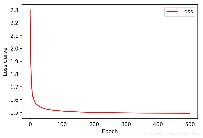
y_t = torch.from_numpy(y).type(torch.LongTensor)训练模型,迭代500次,并画出损失函数曲线和分类准确性曲线。
best_precision = 0
train_loss_curve =[]
train_precision_curve =[]
for epoch in range(500):
    model.train()
    y_pred = model(X_t)
    loss = criterion(y_pred, y_t)
    print(epoch, loss.item())
    optimizer.zero_grad()
    loss.backward()
    optimizer.step()
    train_loss_curve.append(loss.item())
    model.eval()
    y_pred = model(X_t).detach().numpy()
    y_pred = np.argmax(y_pred, axis=1)
    precision = np.mean(y_pred == y) * 100
    train_precision_curve.append(precision)
    if precision > best_precision:
        best_precision = precision
损失函数变化曲线:
准确率变化曲线
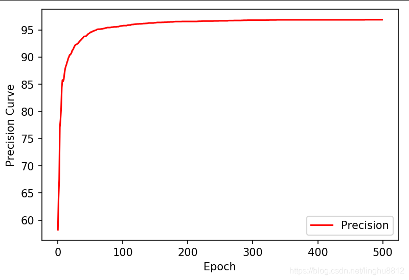
最终训练集上结果的最佳准确率为96.88%。
4.其他尝试
4.1修改Linear层的初始化权重
修改不同的权重初始化方法,查看最终可以达到的最佳准确率
| Initial | Precision | 说明 |
|---|---|---|
| constant_,0 | 96.88% | 初始化为常数 |
| uniform_ | 87.56% | 均匀分布初始化 |
| normal_ | 77.5% | 正态分布初始化 |
| eye_ | 96.92% | 对角线初始化 |
| xavier_uniform_ | 87.62% | xavier均匀分布 |
| xavier_normal_ | 96.86% | xavier正态分布 |
| kaiming_uniform_ | 96.86% | kaiming均匀分布 |
| kaiming_normal_ | 87.48% | kaiming正态分布 |
| orthogonal_ | 87.56% | 正交矩阵 |
如上表所示,可以看出,使用constant_,eye_,xavier_normal_和kaiming_uniform_这几种初始化方法效果最好。
4.2修改weight_decay值
修改不同的weight_decay值,查看最终可以达到的最佳准确率,准确率随weight_decay变化结果如下表所示。
| weight_decay | precision |
|---|---|
| 0 | 96.88% |
| 1e-5 | 96.78% |
| 2e-5 | 96.92% |
| 5e-5 | 96.56% |
| 1e-4 | 96.02% |
| 2e-4 | 94.96% |


 被折叠的 条评论
为什么被折叠?
被折叠的 条评论
为什么被折叠?
 到【灌水乐园】发言


