Matlab reconstruct signal form sample points, convulsion

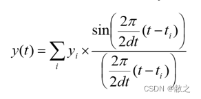
Usually we describe reconstruction as interpolation, and there are many approaches to reach it. In this article, I introduce a new method- convulsion

Main

• signal function
  $f(x)=sin(15\pi x+\pi /10)$

• Convulsion Method
  

• Description of code
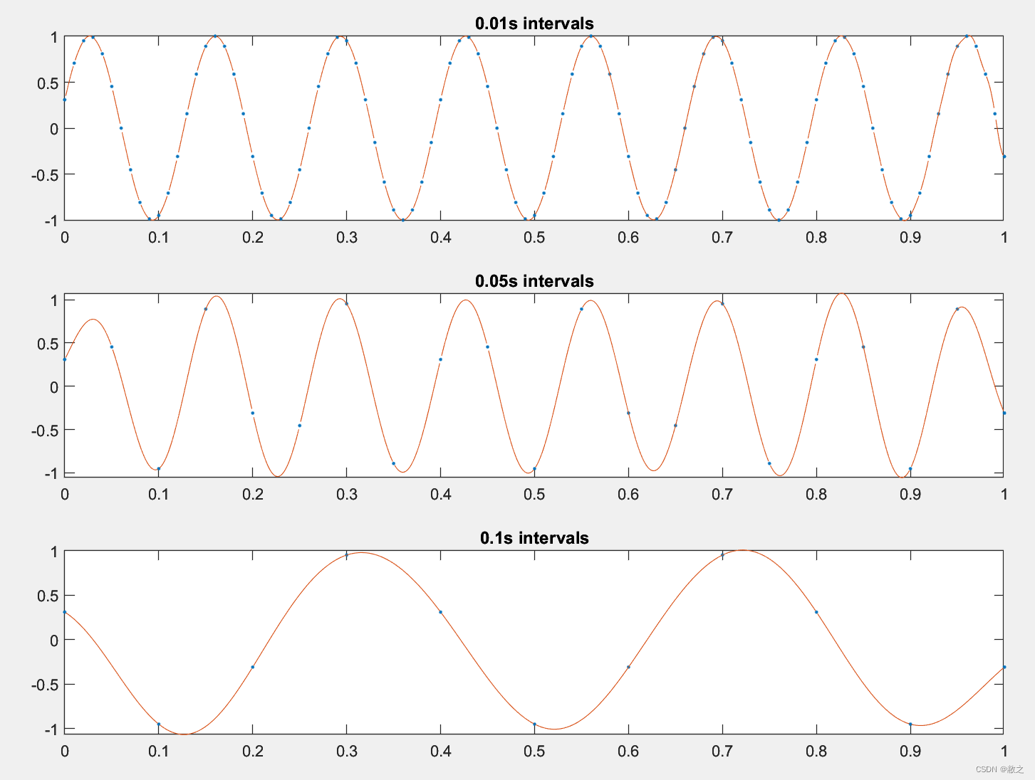
  In this practice, I tested 3 different sample frequencies: 100, 20 and 10 Hz respectively. And the reconstruct frequency is 1000 Hz. As the signal function shows above, the signal frequency is 7.5 Hz.

• Matlab code

clc;
clear;
sP=0.01;
sX=[0:sP:1];
sY=sin(15*pi*sX+pi/10);
sR=0.001;
xR=[0:sR:1];
N = length(sX);         % number of samples
yR = zeros(size(xR));
for t = 1:length(xR)
    for n = 0:N-1
        yR(t) = yR(t) + sY(n+1)*sin(pi*(xR(t)-n*sP)/sP)/(pi*(xR(t)-n*sP)/sP);
    end
end
subplot(3,1,1)
plot(sX,sY, ".");
hold on;
plot(xR,yR, "-");
title('0.01s intervals')

sP=0.05;
sX=[0:sP:1];
sY=sin(15*pi*sX+pi/10);
sR=0.001;
xR=[0:sR:1];
N = length(sX);         % number of samples
yR = zeros(size(xR));
for t = 1:length(xR)
    for n = 0:N-1
        yR(t) = yR(t) + sY(n+1)*sin(pi*(xR(t)-n*sP)/sP)/(pi*(xR(t)-n*sP)/sP);
    end
end
subplot(3,1,2)
plot(sX,sY, ".");
hold on;
plot(xR,yR, "-");
title('0.05s intervals')

sP=0.1;
sX=[0:sP:1];
sY=sin(15*pi*sX+pi/10);
sR=0.001;
xR=[0:sR:1];
N = length(sX);         % number of samples
yR = zeros(size(xR));
for t = 1:length(xR)
    for n = 0:N-1
        yR(t) = yR(t) + sY(n+1)*sin(pi*(xR(t)-n*sP)/sP)/(pi*(xR(t)-n*sP)/sP);
    end
end
subplot(3,1,3)
plot(sX,sY, ".");
hold on;
plot(xR,yR, "-");
title('0.1s intervals')

• Result

• analysis

1. As result shown above, the first and second graph revice the original signal perfectly with correct frequency and amplitude. But the frequency of the third one is not right due to the sample frequency (10Hz) is lower than 2 times of signal its original frequency (15Hz). Hence, the reconstruct signal has lower frequency.