Matlab project1 phase 2&3 - Minimum Snap/Jerk and A* Algorithm ＜Experiment recording＞

Preface:This article is written for a nifty girl who I cherish.

(0)Minimum Snap/Jerk Trajectory Generation

(0.0)Theory

Handle problem

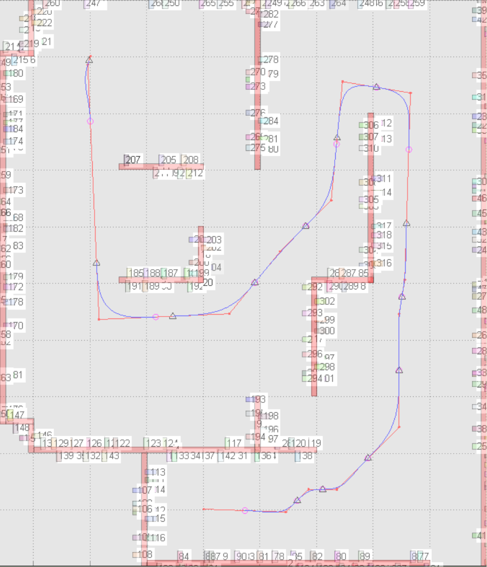
空间中有少量路径点，试图构建一条连续的路径，这条路径经过我们所给的少数路径点，使得无人机能够平滑地飞过这个路径

Method

• 多项式有很好的特性，比如计算方便（可以用矩阵表示），可拟合高阶曲线，所以多项式拟合路径；
• 考虑到路径可能很复杂，如果整个路径用一个多项式表示，那么就会使得拟合路径的多项式阶数很高，并且不能处理闭环路径；所以我们采用每个路径点之间用一个多项式拟合；
• 并且为了使得拟合曲线满足函数的“不可一对多”，我们拟合的是一个参数方程，其自变量为时间

On drone

在无人机中，我们往往考虑要是得最小化加加速度(jerk)或者最小化加加加速度(snap)

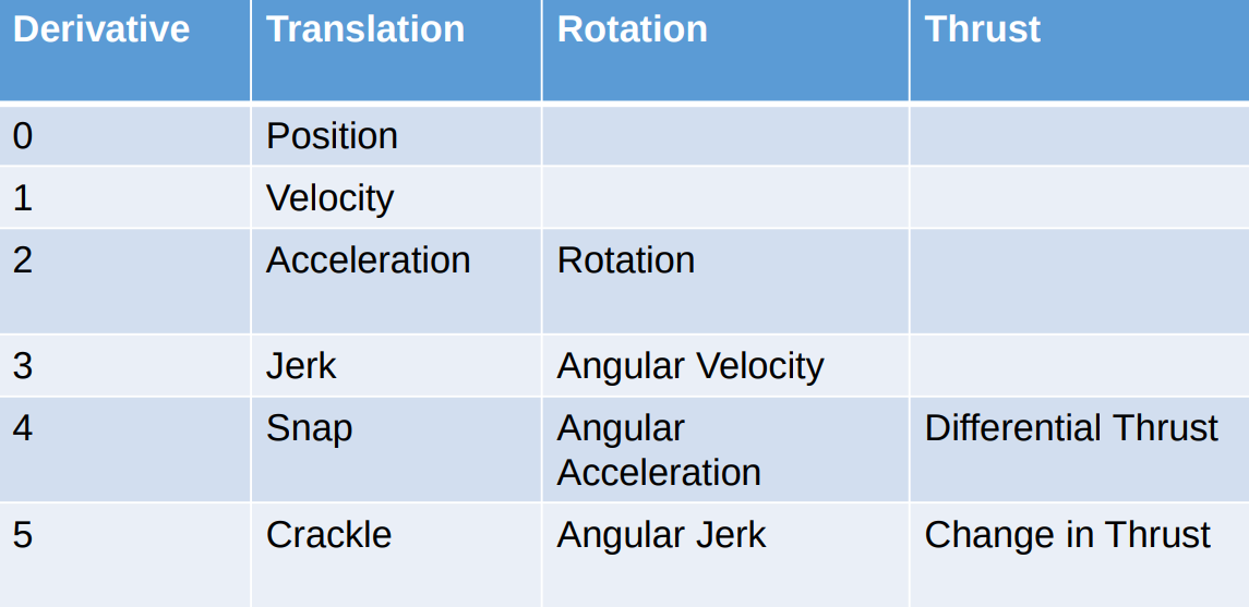
• 其中
• 最小化速度(jerk)保证了无人机飞行路径最短
• 最小化加加速度(jerk)保证了无人机飞行的稳定性（因为加加速度与无人机pitch，roll轴的角速度成真比）
• 加加加速度(snap)保证了无人机的耗能最小（因为）

Problem defination

Target：最小化加加速度(jerk)或者加加加速度(snap)
Constraints：对初始结束位置速度加速度的约束，对位置点的约束，对连续的约束

这个可以转换为一个二次规划的问题，在Matlab中通过quadprog函数对其进行求解

quadprg:
$$x=quadprog(H,f,A,b,Aeq,beq,lb,ub)$$
其中：

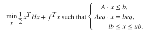
可见目标优化函数需要写作二次型的形式，约束函数写作矩阵乘向量的形式

Problem sloving

Target:

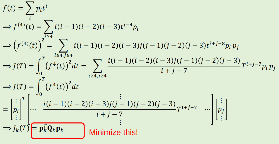
对于5次多项式的轨迹，定义优化函数：
$$\begin{gathered} min{\int }_0^T(p(t{)}^{(3)}{)}^{2}dt \\ =min\sum _{i=1}^k{\int }_{t_{i-1}}^{t_i}(p(t{)}^{(3)}{)}^{2}dt \\ =min\sum _{i=1}^k{\int }_{t_{i-1}}^{t_i}([0,0,0,6,24t,60t^2]\left[\begin{array}{c}{p}_{i0}\\ p_{i1}\\ p_{i2}\\ p_{i3}\\ p_{i4}\\ p_{i5}\end{array}\right]{)}^{2}dt \\ =min\sum _{i=1}^k{\int }_{t_{i-1}}^{t_i}([0,0,0,6,24t,60t^2]P_i{)}^{2}dt \\ =min\sum _{i=1}^k{\int }_{t_{i-1}}^{t_i}([0,0,0,6,24t,60t^2]P_i{)}^T([0,0,0,6,24t,60t^2]P_i)dt \\ =min\sum _{i=1}^k{P}_i^T{\int }_{t_{i-1}}^{t_i}[0,0,0,6,24t,60t^2{]}^T[0,0,0,6,24t,60t^2]dt{P}_i \\ =min\sum _{i=1}^k{P}_i^T{Q}_i{P}_i \end{gathered}$$
可见$Q_i$是一个矩阵，那么要把所有$Q_i$合并起来，又相互不参数干扰，就只有把所有矩阵用主角线把他们串起来：
$$\left(\begin{array}{ccccc}{P}_1& 0& \cdots & 0& 0\\ 0& P_2& \cdots & 0& 0\\ ⋮& ⋮& \ddots & 0& 0\\ 0& 0& 0& p_{k-1}& 0\\ 0& 0& 0& 0& p_k\end{array}\right)$$

matlab 中计算单个$Q_i$函数可以是：

% n:polynormial order
% r:derivertive order, 1:minimum vel 2:minimum acc 3:minimum jerk 4:minimum snap
% t1:start timestamp for polynormial
% t2:end timestap for polynormial
function Q = computeQ(n,r,t1,t2)
syms x real;
a=x;
%generate simple polynormial like: x+x^2+x^3+x^4+x^5+x^6
for i=1:n
    a(end+1)=a(end)*x;
end
a=diff(a,r+1);
a1(x)=a'*a;
a2=int(a1(x),x);
Q=double(subs(a2,t2)-subs(a2,t1));

Equation Constraints:

有三类约束：

• 起始点终点位置、速度、加速度约束
  位置约束：
  $$\begin{gathered} [1,t,t^2,t^3,t^4,t^5]{\vec{P}}_1=x_0 \\ [1,t,t^2,t^3,t^4,t^5]{\vec{P}}_e=x_e \end{gathered}$$
  速度约束：
  $$\begin{gathered} [0,1,2t,3t^2,4t^3,5t^4]{\vec{P}}_1=v_0 \\ [0,1,2t,3t^2,4t^3,5t^4]{\vec{P}}_e=v_e \end{gathered}$$
  加速度约束：
  $$\begin{gathered} [0,0,2,6t,12t^2,20t^3]{\vec{P}}_1=a_0 \\ [0,0,2,6t,12t^2,20t^3]{\vec{P}}_e=a_e \end{gathered}$$
  matlab先求多项式，再求导，代入$t$值，列出矩阵与向量
  有六个方程
• 中间点位置约束
  $$[1,t,t^2,t^3,t^4,t^5]{\vec{P}}_n=x_n$$
  其中$n=2,3,4...k-2,k-1$
  有k-2个方程
• 中间点连续约束
  位置连续：
  $$\begin{gathered} [1,t,t^2,t^3,t^4,t^5]{\vec{P}}_{n-1}=[1,t,t^2,t^3,t^4,t^5]{\vec{P}}_n \\ 即：[1,t,t^2,t^3,t^4,t^5]{\vec{P}}_{n-1}-[1,t,t^2,t^3,t^4,t^5]{\vec{P}}_n=0 \\ 即：[1,t,t^2,t^3,t^4,t^5,-1,-t,-t^2,-t^3,-t^4,-t^5]\left[\begin{array}{c}{\vec{P}}_{n-1}\\ {\vec{P}}_n\end{array}\right]=0 \end{gathered}$$
  同理速度连续：
  $$[0,1,2t,3t^2,4t^3,5t^4,-0,-1,-2t,-3t^2,-4t^3,-5t^4]\left[\begin{array}{c}{\vec{P}}_{n-1}\\ {\vec{P}}_n\end{array}\right]=0$$
  同理加速度连续：
  $$[0,0,2,6t,12t^2,20t^3,-0,-0,-2,-6t,-12t^2,-20t^3]\left[\begin{array}{c}{\vec{P}}_{n-1}\\ {\vec{P}}_n\end{array}\right]=0$$
  这里在matlab中就要注意排列约束的时候要按照顺序排列，这样才能保证中间点约束
  有(k-2)x3个方程
  综上：一共有(k-2)x4+6个约束方程

(0.1)codes

code

(1)A* algorithm

(1.0)Description

初始化

初始化Map矩阵，保存地图信息，1为障碍，0不是障碍
初始化gScore矩阵，保存分数信息，设置开始点为1，其余为无穷
初始化expanded矩阵，保存访问信息，设置全为0
初始化parents矩阵，用于保存节点的父节点信息，易于回溯
初始化queue矩阵，用于保存待访问节点，内部只有初始节点
while (queue不为空)
	从queue中取出g+h分数最小的节点p
	标记节点p于expanded为1
	把p节点从queue中删除
	找出p节点邻居节点中满足以下条件的节点ps:
		非障碍物，没有越界，没有被访问过
	将这些节点ps的父节点parents设置为p
	如果ps中含有终点，跳出while循环
如果终点没有父节点
	没有可达路径
如果终点有父节点
	从parents中向上不断寻找父节点，直到访问到开始节点，记录路径

(1.1)coding with matlab

• 于matlab中数组中添加一个向量

queue(end+1,:)=map(1,:);

• 于matlab中删除一个向量

queue(minIndex,:)=[];

• matlab 反转一个向量

Optimal_path=flip(Optimal_path)

(1.2)codes

code

(2)More things

(2.0)Minimum polynomial degree

WHY?

(2.1)Polynomial Trajectories - corridor

• Problems: 得到的路径可能会撞到障碍物，我们需要设置一定的可通行区域，保证无人机于区域内飞行
• Methods: 在可行路径中添加采样点，设置不等式约束，保证采样点都满足不等式约束
  即:
  $$[1,t,t^2,t^3,t^4,t^5]p_j<p(j)+r$$
  $$[-1,-t,-t^2,-t^3,-t^4,-t^5]p_j<-p(j)-r$$
  $p(j)$为采样点的位置，$p_j$是采样点段的多项式参数，时间是到达该点的时间
  实际还有可行性检测（feasibility check），确保速度，加速度能够达到

(2.2)Polynomial Trajectories - divide time

• Problems: 现有时间分配不合理，我们约束是每一维度的速度相同，但速度叠加后速度就不同了
• Methods: 匀速分配，梯形分配

(2.3)Polynomial Trajectories - Closed form

• Problems: 二次规划求解速度慢
• methods: 闭式求解(只能有等式约束)，只需要矩阵运算求解

(3)Reference

https://blog.youkuaiyun.com/q597967420/article/details/76099491